Negative-Ion Influence on Precipitation
Preamble
This document is being developed by the Senior Engineer of AscenTrust, LLc. at the request of Mr. Arun Savkur for the benefit of WeatherTec.
The WeatherTec Ionization Technology has a proven track record in increasing the annual average amount of precipitation in the land area adjacent to the Emitter. The negative-ions produced at the Emitter, injected into the atmosphere, rise to the convective cloud layer acting as Cloud Condensation Nuclei, to increase natural rainfall development.
The Senior Engineer has been tasked with the development of a mathematical model linking the onset of precipitation, within an identifiable land area surrounding the Electrodynamic Device, which wil be referred to as the Emitter, on the surface layer of the planetary boundary layer, to the local electrodynamic State of the Fair Weather Voltage Gradient to the lower cloud layer of the troposphere. This model will introduce thermodynamic, statistical mechanical, fluid mechanics,turbulence and vortex theory into the conceptual framework for a realistic atmospheric model of the posibility of enhancing the amount of precipitation within the footprint of our point source of Negative-Ions.
1. The Senior Engineer is a Graduate of Electrical and Computing Engineering and Graduated with distinction in 1969. His thesis topic, for his masters degree, was the development of a theoretical model of non-linear laser interactions, to promote ion heating in magnetized plasma. It is therefore natural that the Senior Engineer would concentrate his efforts on the interactions of the Global Electrical Circuit, fair Weather Electrostatic Gradient and the diurnal behavior of the magnetosphere, to provide the theoretical background for the interaction of negative-ions with fair-weather clouds to enhance precipitation at the footprint of the Planetary Boundary Layer
2. Definition of terms in meteorology and atmospheric physics is variable and inconsistant. In order to mitigate this problem we will be using the Glossary of Meteorology belonging to the American Meteorology Society.
3. This document is being developed to provide the theoretical and mathematical basis supporting the use of the negative-ions Emitter technology belonging to Weathertec to increase precipitation. The models being developed include thermodynamic and electrodynamic modeling
4. This document will provide a fairly extensive introduction to the dipole structure of the water moleacule and the increase in individual dipole moment, of the water moleacule in chemically bonded series of water moleacules. The polar characteristics of water are one of the most important properties of the water moleacule. The dipolar structure of the water moleacule is responsible for the large surface tension ascribed to a water droplet that allows the water aerosol to form clouds.
5. This document includes an introduction to the subjects of the Global Electrical Circuit, the Fair Weather Voltage Gradient and Atmospheric Electrodynamic. Atmospheric electrification is responsible for the creation of charged Cloud Condensation Nuclei. These CCN are responsible for the creation of Thunderstorms. The Weathertec Emitter creates an negative-ion aerosol at the surface of the earth to modify the local micrometeorological Microphysics, and thereby create precipitation.
6. This webpage is in a state of ongoing development and new material will appear from time to time as the workload permits.
7. The text and mathematical equations in this document are renderred in HTML using a web-based Latex and Javascript renderring engine.
Part One: Models and Reality
The Academic idea that modelling and simulations can bring us to an understanding of reality is false. Certainly, modelling has become an essential and inseparable part of many scientific disciplines, each of which has its own ideas about specific types of modelling. The following was said by John von Neumann:
... the sciences do not try to explain, they hardly even try to interpret, they mainly make models. By a model is meant a mathematical construct which, with the addition of certain verbal interpretations, describes observed phenomena. The justification of such a mathematical construct is solely and precisely that it is expected to work—that is, correctly to describe phenomena from a reasonably wide area.
A scientific model seeks to represent natural phenomena, and physical processes in a logical and objective way. All models are simplified simulation of reality that, despite being approximations, can be extremely useful. Building and disputing models is fundamental to the Academic enterprise. Complete and true representation are impossible, but Academics debate often concerns which is the better model for a given task.
Attempts are made by Academics to formalize the principles of the empirical sciences in the same way logicians axiomatize the principles of logic. The aim of these attempts is to construct a formal system that will not produce theoretical consequences that are contrary to what is found in reality. Predictions or other statements drawn from such a formal system mirror or map the real world only insofar as these scientific models are true.
For the atmospheric scientist, the global models used are rendered in software algorithms to simulate, visualize and gain intuition about the atmospheric phenomenon, or process being represented.
Part 1.1: Mathematical Models
A mathematical model is an abstract description of a concrete system using mathematical concepts and language. The process of developing a mathematical model is termed mathematical modeling. Mathematical models are used extensively in atmospheric physics, in the natural sciences and in engineering.
Mathematical models can take many forms, including dynamical systems, statistical models or differential equations. These and other types of models can overlap, with a given model involving a variety of abstract structures. In general, mathematical models may include logical models. In many cases, the quality of a scientific field depends on how well the mathematical models developed on the theoretical side agree with results of repeatable experiments. Lack of agreement between theoretical mathematical models and experimental measurements often leads to important advances as better theories are developed.
In the physical sciences, a traditional mathematical model contains most of the following elements:
- Governing equations
- Supplementary sub-models
- Defining equations
- Constitutive equations
- Assumptions and constraints
- Initial and boundary conditions
- Classical constraints and kinematic equations
Part 1.2: Mathematical Model Classification
Linear Vs. Nonlinear: If all the operators in a mathematical model exhibit linearity, the resulting mathematical model is defined as linear. A model is considered to be nonlinear otherwise. The definition of linearity and nonlinearity is dependent on context, and linear models may have nonlinear expressions in them. For example, in a statistical linear model, it is assumed that a relationship is linear in the parameters, but it may be nonlinear in the predictor variables. Similarly, a differential equation is said to be linear if it can be written with linear differential operators, but it can still have nonlinear expressions in it. In a mathematical programming model, if the objective functions and constraints are represented entirely by linear equations, then the model is regarded as a linear model. If one or more of the objective functions or constraints are represented with a nonlinear equation, then the model is known as a nonlinear model.
Linear Structure: implies that a problem can be decomposed into simpler parts that can be treated independently and/or analyzed at a different scale and the results obtained will remain valid for the initial problem when recomposed and rescaled.
Nonlinearity: Nonlinearity, even in fairly simple systems, is often associated with phenomena such as chaos and irreversibility. Although there are exceptions, nonlinear systems and models tend to be more difficult to study than linear ones. A common approach to nonlinear problems is linearization, but this can be problematic if one is trying to study aspects such as irreversibility, which are strongly tied to nonlinearity.
Static Vs. Dynamic: A dynamic model accounts for time-dependent changes in the state of the system, while a static (or steady-state) model calculates the system in equilibrium, and thus is time-invariant. Dynamic models typically are represented by differential equations or difference equations.
Explicit Vs. Implicit: If all of the input parameters of the overall model are known, and the output parameters can be calculated by a finite series of computations, the model is said to be explicit. But sometimes it is the output parameters which are known, and the corresponding inputs must be solved for by an iterative procedure, such as Newton's method or Broyden's method. In such a case the model is said to be implicit. For example, a jet engine's physical properties such as turbine and nozzle throat areas can be explicitly calculated given a design thermodynamic cycle (air and fuel flow rates, pressures, and temperatures) at a specific flight condition and power setting, but the engine's operating cycles at other flight conditions and power settings cannot be explicitly calculated from the constant physical properties.
Discrete Vs. Continuous: A discrete model treats objects as discrete, such as the particles in a molecular model or the states in a statistical model; while a continuous model represents the objects in a continuous manner, such as the velocity field of fluid in pipe flows, temperatures and stresses in a solid, and electric field that applies continuously over the entire model due to a point charge.
Deterministic Vs. probabilistic (stochastic): A deterministic model is one in which every set of variable states is uniquely determined by parameters in the model and by sets of previous states of these variables; therefore, a deterministic model always performs the same way for a given set of initial conditions. Conversely, in a stochastic model—usually called a "statistical model"—randomness is present, and variable states are not described by unique values, but rather by probability distributions.
Deductive, inductive, or floating: A deductive model is a logical structure based on a theory. An inductive model arises from empirical findings and generalization from them. The floating model rests on neither theory nor observation, but is merely the invocation of expected structure. Application of mathematics in social sciences outside of economics has been criticized for unfounded models. Application of catastrophe theory in science has been characterized as a floating model.
Part Two: Prototypes
A prototype is the early physical model of a product built to test the theoretical validity of the model. It is a term used in a variety of contexts, including semantics, design, electronics, and software programming. A prototype is generally used to evaluate a new design to enhance precision by system analysts and users. Prototyping serves to provide specifications and acquire data for a real, working system rather than a theoretical one. In some design workflow models, creating a prototype (a process sometimes called materialization) is the step between the formalization and the evaluation of an idea. In the case of ionization of air and water moleacules we have developed several different prototypes for different applications
Prototypes explore the different aspects of an intended design:
1. A proof-of-principle prototype serves to verify some key functional aspects of the intended design, but usually does not have all the functionality of the final product.
2. A working prototype represents all or nearly all of the functionality of the final product.
3. A visual prototype represents the size and appearance, but not the functionality, of the intended design. A form study prototype is a preliminary type of visual prototype in which the geometric features of a design are emphasized, with less concern for color, texture, or other aspects of the final appearance.
4. A user experience prototype represents enough of the appearance and function of the product that it can be used for user research.
5. A functional prototype captures both function and appearance of the intended design, though it may be created with different techniques and even different scale from final design.
6. A paper prototype is a printed or hand-drawn representation of the user interface of a software product. Such prototypes are commonly used for early testing of a software design, and can be part of a software walkthrough to confirm design decisions before more costly levels of design effort are expended.
Part Three: Theoretical Model
This document was commmissioned to the elucidation of an old theory of water droplet nucleation put forward in the early part of the twentieth Century by the American Meteorologist, Charles Thomson Rees Wilson. Wilson was a Scottish physicist and meteorologist who won the Nobel Prize in Physics for his invention of the cloud chamber. Despite Wilson's great contribution to particle physics, he remained interested in atmospheric physics, specifically atmospheric electricity, for his entire career. Wilson developed the first theory of the electrification of thunderstorm clouds.
Clouds are formed by the lifting of damp air (from the planetary surface) which then cools Adiabatically by expansion as it encounters falling pressure at higher levels of the troposphere. The relative humidity consequently rises and eventually the air becomes saturated with water vapor. Further cooling produces a supersaturated vapor. In this supersaturated layer the water condenses on to aerosols, present in the upper troposphere. These aerosol can be carbon based (soot or flyash), silica based (sand), solvated sea salt (Sodium Chloride) or positively or negatively charged ions. The condensation of water vapor on these aerosols, suspended in the middle to upper troposphere, forms a cloud composed of minute water droplets.
Classical models of cloud seeding are based on the injection of aerosols above or below the cloud layer. These aerosols, generally consisting of sea salt, sulphates, silver iodine or dry ice (Carbon dioxide).
Our Weather Modification Technology creates negative-ions aerosols at the surface layer of the Planetary boundary layer of the atmosphere. These aerosols are then delivered to the underside of the saturated layer of the fair weather cloud.
The physics of our model will be centered around the thermodynamic and the electrodynamic interaction of clouds with the global Electrical Circuit and its manifestation in the Earth Boundary Layer.
The three important most important components required for the dynamics of water droplet formation are water, aerosols and ions.
Our analyses of the microphysics of the atmospheric surface boundary layer surrounding our negative ion emitter will include the physics of the corona discharge from a high voltage source. The is methodology for the creation of raindrops in the upper part of the troposphere
This document will concentrate on the electrodynamic interaction of water moleacules with aerosols in the formation of the nucleation sphere required to create water droplets in the upper part of the troposphere
At the Surface Layerof the Planetary Boundary Layer the microphysics of the prototype will include the interaction of the corona electrons required to create negative ions adjacent to the prototype. From the buildup of negative ions at the footprint of the prototype we will present the point source physics for the migration of the negative ions by convective and electric potential forces to the upper layer of the troposphere.
Part Four: Summary of Document
Section One: A brief introduction to Weather Systems with an emphasis on the interactions of local ionization on micrometerology. Our negative-ion Emitter is located on the surface of the earth, in what is commonly referred to the Surface Layer of the Planetary Boundary Layer. The geographic location of the emitter defines the geographic center of the area which we will refer to as the Zone of Precipitation of our weather modification atmospheric model.
This document will include enough of the elements of mathematical physics to allow the reader to follow the mathematical modeling, both at large scale and at the microscale or local scale and to understand the theoretical modeling of our Weather Modification Technology. We will be discussing the physics of negative-ion creation on the surface of the earth and the interaction of these negative-ion within the planetary boundary layer. The interaction of negative-ions with the surface voltage gradient and the planetary magnetic field at the boundary layer creates a vortex. The creation and maintenance of the vortex attached to the boundary layer of the earth creates a negative-ion aerosol plume. The aerosol plume rises to the cloud formation layer of the troposphere where the negatively charged ions form the central core of Cloud Condensation Nuclei.
Section Two: Introduction to Thermodynamic Concepts
The thermodynamic concepts which we are interested in are: Internal Energy, enthalpy, Entropy, Helmholtz Free Energy, Gibbs Free Energy, etc. These thermodynamic properties will be introduced as belonging to a thermodynamic system. The thermodynamic properties of the system define the State of the system. This introduction to thermodynamic concepts will be done under the ideal notion of a Closed Systems. Only the thermodynamic properties of perfect gases will be addressed in this section with the clear understanding that all systems considered in atmospheric thermodynamics are open systems and are therefore difficult to analyse using these classic thermodynamic concepts.
Section Three: Introduction to Classical Mechanics
The scope of this short introduction to classical mechanics will be kept within the narrow range of the mechanical laws which serve as an introduction to hydrodynamics, quantum mechanical, electrodynamic, magnetohydrodynamic and statistical mechanical theories of the atmosphere and more particularily to cloud physics and the circulation models of the oceans and the atmosphere. The classical mechanical concepts which we are interested in are: Neutonian Mechanics, Lagrangian Mechanics and Hamiltonian Mechanics
Section Four: Introduction to Hydrodynamics
The defining property of fluids, including atmospheric gases and water, lies in the ease in which they can be deformed. The fact that relative motion of different elements of a portion of fluid can, and in general does, occur when forces act on the fluid gives rise to the study of hydrodynamics. In this section we will outline some elementary concepts of fluid mechanics which is pertinent to atmospheric studies. In addition we will discuss conservation laws, including mass, momentum and energy. We will also introduce the Lagrangian and Eulerian specifications. Finally we will introduce concepts such as Newtonian versus non-newtonian fluids and we will introduce the concept of turbulent flow in the atmosphere.
Section Five: Introduction to Electrodynamics
The surface of the earth is a good conductor of electricity. The ocean, because of the inclusion of sodium chloride, an electrolyte, has a conductivity which is three orders of magnitude higher that the surfaace conductivity. We are therefore required to include a brief introduction to electrostatics, magnetostatic and electrodynamics to a sufficient level to grasp the main arguments concerning the creation of Charged Aerosols in the troposphere. These Cloud Condensation Nuclei form the core concept of nucleation which leads to precipitation.
Section Six: Introduction to magnetohydrodynamics
which is pertinent to atmospheric studies. The magnetohydrodynamic forces of the solar winds are extremely important in the creation and maintenance of the Global Electrical Circuit. We will also be concerned with the geomagnetic influence on thunderstorms.
Section Seven: Introduction to Electrochemistry
This section contains an analysis of those aspects of electrochemistry which are required to understand the essentials of the electrochemical interaction at the interface of the emitter to atmosphere and to follow the pathway to the creation of the small Aerosols responsible for the creation of cloud condensation nuclei.
Section Eight: Introduction to the fundamentals of Quantum Mechanics
Many of the theoretical components of our modelling involve quantum Mechanical models. This section is a brief overview of the quantum mechanical concepts required for a proper analysis of the interaction of electrons with atmospheric Oxygen for the initial formation of Aerosols at the planetary surface layer.
Section Nine: Introduction to Surface States
This section contains an outline of the Basic Theory of Surface States. The analysis will quantum mechanical,thermodynamic, electrodynamic and electrochemical properties of the surface states of liquid water. These surface states are responsible for surface tension at the interface of water and the atmosphere.
Section Ten: A concise introduction to Nanoclusters and Microparticles the nature and dynamical properties of Aerosols. An aerosol is defined as a suspension system of solid or liquid particles in a gas. In this document we will be discussing the interactions of aerosols with the planetary electrical circuit in the consolidation of water droplets to create precipitation.
Section Eleven: A detailed introduction to the properties of water. This section contains a detailed analysis of the thermodynamic, electrodynamic and electrochemical properties of the water moleacule which makes this highly polar moleaculer one of the most important and unique substance in the biosphere.
Section Twelve: A detailed discussion of Aerosols. We will be discussing the nature and dynamical properties of Aerosols. An aerosol is defined as a suspension system of solid or liquid particles in a gas. In this document we will be discussing the interactions of aerosols with the planetary electrical circuit in the consolidation of water droplets to create precipitation.
Section Thirteen: consists of an introduction to Statistical Physics and Statistical Mechanics as a precursor to our study of turbulence and the theory of Vorticies
Section Fourteen: consists of an introduction to the topics related to the earth. These topics include the analysis of the earth as a Geoid, the earth's gravitation field, the earth's magnetic field and the earth's static electric gradient.
Section Fifteen: consists of an introduction to the earth's atmosphere. This introduction includes the general clasification of the layers of the atmosphere. The atmosphere will be discussed in terms of the troposphere, the stratosphere, the mesosphere, the thermosphere, the exosphere and the ionosphere. We will also include a brief discussion of the ozone layer, the homosphere, the hydrosphere and the earth's boundary layer.
Section Sixteen: consists of an introduction to Turbulence. Turbulence or turbulent flow is fluid motion characterized by chaotic changes in pressure and flow velocity. All interactions in the atmosphere are classified as turbulent. The creation of vortices in the planetary boundary layer is a very important theoretical part of our model.
Section Seventeen: consists of an introduction to Dynamic meteorology. Dynamic meteorology is the study of those motions of the atmosphere that are associated with the production of the circulation models, including the dynamics of air and moisture. For all such motions the discrete molecular nature of the atmosphere can be ignored, and the atmosphere can be regarded as a continuous fluid medium.
Section Eighteen: consists of an introduction to the existing models of hydrodynamic turbulence. We will only outline the models which are useful for the elucidation of our theoretical model of enhancing precipitation through negative-ion interactions in the base of low level clouds comenly referred to as fair weather clouds.
Section Nineteen: consists of a preliminary discussion of two of the most important planetary processes which are involved in the creation of clouds, precipitation and thunderstorms. The first is referred to as Global Circulation Model and the second is Global Electrical Circuit and the final part will refer to the Planetary Magnetohydrodynamic System.
Section Twenty: consists of an introduction to Clouds, their classification and their role in precipitation. Terrestrial clouds can be found throughout most of the homosphere, which includes the troposphere, stratosphere, and mesosphere. Within these layers of the atmosphere, air can become saturated as a result of being cooled to its dew point or by having moisture added from an adjacent source. The moisture then coalesces to become droplets of water. These droplets are the major constituent of clouds.
Section Twenty-One: consists of an introduction to Electrical effects on Fair Weather Clouds have been proposed to occur via the ion-assisted formation of ultra-fine aerosol.
Section Twenty-Two: consists of an introduction to Cloud Condensation Nuclei (CCNs). CCN are small particles typically 0.2 µm, or one hundredth the size of a cloud droplet on which water vapour begins to condense to form a droplet. These cloud condensation nuclei then form the basis for the formation of raindrops in the upper part of the Troposphere. When the droplets reach a size of $ {\displaystyle 100 \mu} $ they fall to earth as precipitation.
Section Twenty-Three: consists of a discussion of the different processes by which nuclear droplets may attain radii of several microns and so form a cloud. We will discuss the diffusion of water vapour to and its condensation upon their surface, and coalescence of droplets relative to each other by virtue of Brownian Motion, small-scale turbulance, electrical forces, and differential rates of fall under gravity.
Section Twenty-Four: consists of an introduction to the Planetary Boundary Layer and the Surface Boundary Layer which form the lower part of the atmosphere in direct contact to the earth. It is in the surface layer of the atmospheric boundary layer that our prototypes injects negative ions into a vortex tube (aerosol plume) which allows the ions to migrated upwards and interact with the layer of low clouds to enhance the production of CCN and therefore increase the probability of presipitation.
Section Twenty-Five: consists of an introduction to The first prototype produces free electrons through corona discharge from a high-voltage copper cathode.
Section Twenty-Six: consists of an introduction to Flow of aerosols in the form of negative-ions, charged water droplets, vapor or smoke released into the air at a very small altitude in surface layer of the planetary boundary layer. Plumes are of considerable importance in the atmospheric dispersion modelling of aerosols comenly refered to as air pollution. There are three primary types of aerosol emission plumes:
Section One: Introduction to Weather Systems and Micrometerology
Weather is the state of the atmosphere, describing for example the degree to which it is hot or cold, wet or dry, calm or stormy, clear or cloudy. On Earth, most weather phenomena occur in the lowest layer of the planet's atmosphere, the Troposphere, just below the Stratosphere. Weather refers to day-to-day temperature, precipitation, and other atmospheric conditions, whereas climate is the term for the averaging of atmospheric conditions over longer periods of time.
Earth's Energy Budget accounts for the balance between the energy that Earth receives from the Sun and the energy the Earth loses back into outer space. Smaller energy sources, such as Earth's internal heat, are taken into consideration, but make a tiny contribution compared to solar energy. The energy budget also accounts for how energy moves through the climate system. Because the Sun heats the equatorial tropics more than the polar regions, received solar irradiance is unevenly distributed. As the energy seeks equilibrium across the planet, it drives interactions in Earth's climate system, i.e., Earth's water, ice, atmosphere, rocky crust, and all living things. The result is the Earth's weather system.
The Solar Wind is a stream of charged particles released from the upper atmosphere of the Sun, called the corona. This plasma mostly consists of electrons, protons and alpha particles with kinetic energy between 0.5 and 10 keV. The composition of the solar wind plasma also includes a mixture of materials found in the solar plasma: trace amounts of heavy ions and atomic nuclei. Superimposed with the solar-wind plasma is the interplanetary magnetic field. The solar wind varies in density, temperature and speed over time and over solar latitude and longitude. Its particles can escape the Sun's gravity because of their high energy resulting from the high temperature of the corona, which in turn is a result of the coronal magnetic field. The boundary separating the corona from the solar wind is called the Alfvén surface.
At a distance of more than a few solar radii from the Sun, the solar wind reaches speeds of 250–750 km/s and is supersonic, meaning it moves faster than the speed of the fast magnetosonic wave. The flow of the solar wind is no longer supersonic at the termination shock. Other related phenomena include the aurora (northern and southern lights), the plasma tails of comets that always point away from the Sun, and geomagnetic storms that can change the direction of magnetic field lines.
Atmospheric motions are characterized by a variety of scales ranging from the order of millimeter to as large as the circumference of the earth at the planetary layer. The corresponding time scales range from: seconds, hours, diurnal or daily and yearly. These scales of motion are generally classified as: micro-, meso-, and macroscales. Sometimes, terms such as local, regional and global are used to characterize the atmospheric scales and the phenomena associated with them.
This document will be mainly concerned with atmospheric physics at the microscale or local scale and we are therefore working in the scope of Micrometeorology.
Micrometeorology is a branch of meteorology which deals with atmospheric phenomena and processes at the lower end of the spectrum of atmospheric physics, which are variously characterized as microscale, small-scale or local-scale processes.
There is a large body of historical research linking the creation of water droplets, in the troposphere, to the existance of negative and positive ions. The existance of ions in the troposphere creates a physical links among clouds, the global atmospheric electrical circuit and cosmic ray ionisation.
The global circuit extends throughout the atmosphere from the planetary surface to the lower layers of the ionosphere. Cosmic rays are the principal source of atmospheric ions away from the continental boundary layer: the ions formed permit a vertical conduction current to flow in the fair weather part of the global circuit. Through the (inverse) solar modulation of cosmic rays, the resulting columnar ionisation changes may allow the global circuit to convey a solar influence to meteorological phenomena of the lower atmosphere.
Electrical effects on non-thunderstorm clouds have been been extensively studied by the Russians and the Germans who have substantially ellucidated the mechanism of ion-assisted formation of ultrafine aerosol, which can grow to sizes able to act as cloud condensation nuclei, or through the increased ice nucleation capability of charged aerosols.
Even small atmospheric electrical modulations on the aerosol size distribution can affect cloud properties and modify the radiative balance of the atmosphere, through changes communicated locally by the atmospheric electrical circuit.
Section Two: Thermodynamics
Our interest in cloud thermodynamics has to do with our approach to the physics of water droplet formation via negative ion creation in the planetary boundary layer and the transport of these ions to the upper part of the troposphere, to form Cloud Condensation Nuclei for condensation of water vapor into water droplets. The thermodynamic function which we will be mainly interested in is the Gibbs Free Energy and we will use the Gibbs free energy to justify the thermodynamic processes which will be outlined below.
When a system is at equilibrium under a given set of conditions, it is said to be in a definite thermodynamic state. The state of the system can be described by a number of state quantities that do not depend on the process by which the system arrived at its state. They are called intensive variables or extensive variables according to how they change when the size of the system changes. The properties of the system can be described by an equation of state which specifies the relationship between these variables. State may be thought of as the instantaneous quantitative description of a system with a set number of variables held constant.
A thermodynamic process may be defined as the energetic evolution of a thermodynamic system proceeding from an initial state to a final state. It can be described by process quantities. Typically, each thermodynamic process is distinguished from other processes in energetic character according to what parameters, such as temperature, pressure, or volume, etc., are held fixed; Furthermore, it is useful to group these processes into pairs, in which each variable held constant is one member of a conjugate pair.
Thermodynamic Processes Important in Atmospheric Physics are:
1. Adiabatic process: occurs without loss or gain of energy by heat Transfer
2. Isenthalpic process: occurs at a constant enthalpy
3. Isentropic process: occurs at constant entropy
4. Isobaric process: occurs at constant pressure
5. Isothermal process: occurs at a constant temperature
6. Steady state process: occurs without a change in the internal energy
Thermodynamic potentials are different quantitative measures of the stored energy in a system. Potentials are used to measure the energy changes in systems as they evolve from an initial state to a final state. The potential used depends on the constraints of the system, such as constant temperature or pressure.
For example, the Gibbs Free energy will be used almost exclusively in our analysis of the thermodynamics of droplet creation and growth in the clouds.
Part 2.1: Background
The use of thermodynamic ideas, in the study of weather and climate, allows us to quantify the movement of energy within the oceans and the atmosphere of the earth. This part of the document will provide an overview of the basic laws of thermodynamics and the thermodynamics processes which we will be using in this document.
We will first state the two laws of thermodynamics which are pertinent to our discussion of the micrometeorology, of the surface area surrounding the negative ion weather modification device, created within the planetary Boundary Layer.
The first law of thermodynamics
The first law of thermodynamics is essentially a version of the law of conservation of energy, adapted for thermodynamic processes. In general, the conservation law states that the total energy of an isolated system is constant; energy can be transformed from one form to another, but can be neither created nor destroyed.
In a closed system (i.e. there is no transfer of matter into or out of the system), the first law states that the change in internal energy of the system (ΔU system) is equal to the difference between the heat supplied to the system (Q) and the work (W) done by the system on its surroundings.
$${\displaystyle { \Delta U_{\rm {system}}=Q-W \label{eq1}}} $$The First Law asserts the existence of a state variable which is usually called: Internal Energy. This internal energy, $ {\displaystyle U} $ along with the volume, $ {\displaystyle V} $ of the system and the mole number, $ {\displaystyle N_i} $ of its chemical constituents will characterizes the macroscopic properties of the systems equilibrium states.
The Second law of thermodynamics
In a reversible or quasi-static, idealized process of transfer of energy as heat to a closed thermodynamic system of interest, (which allows the entry or exit of energy – but not transfer of matter), from an auxiliary thermodynamic system, an infinitesimal increment ($ {\displaystyle \mathrm {d} S}$ ) in the entropy of the system of interest is defined to result from an infinitesimal transfer of heat ( $ {\displaystyle \delta Q}$ ) to the system of interest, divided by the thermodynamic temperature $ {\displaystyle (T)} $ of the system and the auxiliary thermodynamic system:
$${\displaystyle \mathrm {d} S={\frac {\delta Q}{T}}\qquad\,\,\,\,\,\,\,\,\,\,\,\,\,\,\,\,\,\,\,\,\,\,{\text{(closed system; idealized, reversible process)}}.}$$A convenient form of the second law, useful in atmospheric physics, is to state that for any equilibrium system there exists a state function called entropy, $ {\displaystyle S} $ and that this entropy has the property that it is a function of the extensive parameters of a composite system, such that:
$$ {\displaystyle S = S(U, V, N_1 , . . . , N_ r )} $$Where $ {\displaystyle N_i} $ denotes the mole number of the ith constituent. We further assume that the entropy is additive over the constituent subsystems, that it is continuous and differentiable and a monotonically increasing function of the internal energy, $ {\displaystyle U} $ .
We further assume that in the absence of internal constraints the value of the extensive parameters in equilibrium are those that maximize the entropy.
Part 2.2: Fundamental Relations
Are four fundamental equations which demonstrate how the four most important thermodynamic quantities depend on variables that can be controlled and measured experimentally. Thus, they are essentially equations of state, and using the fundamental equations, experimental data can be used to determine sought-after quantities. The relation is generally expressed as a microscopic change in internal energy in terms of microscopic changes in entropy, and volume for a closed system in thermal equilibrium in the following way. $$ {\displaystyle \mathrm {d} U=T\,\mathrm {d} S-P\,\mathrm {d} V\,} $$ Where, $ {\displaystyle U} $ is internal energy, $ {\displaystyle T} $ is absolute temperature, $ {\displaystyle S} $ is entropy, $ {\displaystyle P} $ is pressure, and $ {\displaystyle V} $ is volume.
This is only one expression of the fundamental thermodynamic relation. It may be expressed in other ways, using different variables (e.g. using thermodynamic potentials). For example, the fundamental relation may be expressed in terms of the enthalpy as: $$ {\displaystyle \mathrm {d} H=T\,\mathrm {d} S+V\,\mathrm {d} P\,} $$ In terms of the Helmholtz free energy ($ {\displaystyle F} $ ) as: $$ {\displaystyle \mathrm {d} F=-S\,\mathrm {d} T-P\,\mathrm {d} V\,} $$ and in terms of the Gibbs free energy ($ {\displaystyle G} $ ) as:
$$ {\displaystyle \mathrm {d} G=-S\,\mathrm {d} T+V\,\mathrm {d} P\,} $$Part 2.2.1: Internal Energy
The properties of entropy outlined above, ensure that the entropy function can be used to define the Internal Energy, such that:
$$ {\displaystyle U = U(S, V, N_1 , . . . , N_ r )} $$This expression is sometimes called the Fundamental Relation in energy form. In specific (per unit mole, or unit mass) form, it can be written as:
$$ {\displaystyle u = u(s, v, n_1 , . . . , n_r ) } $$Where $ {\displaystyle n_i = {\frac {N_j}{{\mathrm \sum_j} N_j}}} $ is the mole fraction.
$$ {\displaystyle {\frac {\mathrm {d} P}{\mathrm {d} T}}={\frac {PL}{T^{2}R}}} $$It then follows that:
$$ {\displaystyle \mathrm{d}U = ( \partial U / \partial S)_{V,N_i} dS + (\partial U / \partial V)_{S,N_i} dV + \sum_i (\partial U / \partial N_i)_{S,V} dN_i } $$Part 2.2.2: Entropy
According to the Clausius equality, for a closed homogeneous system, in which only reversible processes take place, $$ {\displaystyle \oint {\frac {\delta Q}{T}}=0.} $$ With $ {\displaystyle T } $ being the uniform temperature of the closed system and $ {\displaystyle \delta Q } $ the incremental reversible transfer of heat energy into that system. That means the line integral $ {\textstyle \int _{L}{\frac {\delta Q}{T}}} $ is path-independent.
A state function $ {\displaystyle S } $ , called entropy, may be defined which satisfies: $$ {\displaystyle \mathrm {d} S={\frac {\delta Q}{T}}.} $$ Entropy Measurement: The thermodynamic state of a uniform closed system is determined by its temperature $ {\displaystyle T } $ and pressure $ {\displaystyle P } $ . A change in entropy can be written as: $$ {\displaystyle \mathrm {d} S=\left({\frac {\partial S}{\partial T}}\right)_{P}\mathrm {d} T+\left({\frac {\partial S}{\partial P}}\right)_{T}\mathrm {d} P.} $$ The first contribution depends on the heat capacity at constant pressure $ {\displaystyle C_P } $ through: $$ {\displaystyle \left({\frac {\partial S}{\partial T}}\right)_{P}={\frac {C_{P}}{T}}.} $$
This is the result of the definition of the heat capacity by $ {\displaystyle \delta Q = C_P dT } $ and $ {\displaystyle T dS = \delta Q } $ . The second term may be rewritten with one of the Maxwell relations:
$$ {\displaystyle \left({\frac {\partial S}{\partial P}}\right)_{T}=-\left({\frac {\partial V}{\partial T}}\right)_{P}} $$And the definition of the volumetric thermal-expansion coefficient: $$ {\displaystyle \alpha _{V}={\frac {1}{V}}\left({\frac {\partial V}{\partial T}}\right)_{P}} $$
So that:
$$ {\displaystyle \mathrm {d} S={\frac {C_{P}}{T}}\mathrm {d} T-\alpha _{V}V\mathrm {d} P.} $$With this expression the entropy $ {\displaystyle S } $ at arbitrary $ {\displaystyle P } $ and $ {\displaystyle T } $ can be related to the entropy $ {\displaystyle S_0 } $ at some reference state at $ {\displaystyle P_0 } $ and $ {\displaystyle T_0 } $ according to:
$$ {\displaystyle S(P,T)=S(P_{0},T_{0})+\int _{T_{0}}^{T}{\frac {C_{P}(P_{0},T^{\prime })}{T^{\prime }}}\mathrm {d} T^{\prime }-\int _{P_{0}}^{P}\alpha _{V}(P^{\prime },T)V(P^{\prime },T)\mathrm {d} P^{\prime }.} $$In classical thermodynamics, the entropy of the reference state can be put equal to zero at any convenient temperature and pressure.
$ {\displaystyle S(P, T) } $ is determined by followed a specific path in the $ {\displaystyle P-T } $ diagram: integration over $ {\displaystyle T } $ at constant pressure $ {\displaystyle P_0 } $ , so that $ {\displaystyle dP = 0 } $ , and in the second integral one integrates over $ {\displaystyle P } $ at constant temperature $ {\displaystyle T } $ , so that $ {\displaystyle dT = 0 } $ . As the entropy is a function of state the result is independent of the path.
The above relation shows that the determination of the entropy requires knowledge of the heat capacity and the equation of state. Normally these are complicated functions and numerical integration is needed.
The entropy of inhomogeneous systems is the sum of the entropies of the various subsystems. The laws of thermodynamics can be used for inhomogeneous systems even though they may be far from internal equilibrium. The only condition is that the thermodynamic parameters of the composing subsystems are (reasonably) well-defined.
Part 2.2.3: Enthalpy
The enthalpy $ {\displaystyle H} $ of a thermodynamic system is defined as the sum of its internal energy and the product of its pressure and volume:
$$ {\displaystyle H = U + pV} $$Where $ {\displaystyle U} $ is the internal energy, $ {\displaystyle p} $ is pressure, and $ {\displaystyle V} $ is the volume of the system.
Enthalpy is an extensive property; it is proportional to the size of the system (for homogeneous systems). As intensive properties, the specific enthalpy $ {\displaystyle h = H/m} $ is referenced to a unit of mass $ {\displaystyle m} $ of the system, and the molar enthalpy $ {\displaystyle H_n} $ is $ {\displaystyle H/n} $ , where $ {\displaystyle n} $ is the number of moles. For inhomogeneous systems the enthalpy is the sum of the enthalpies of the component subsystems:
$$ {\displaystyle H=\sum _{k}H_{k},} $$Where:
- $ {\displaystyle H } $ is the total enthalpy of all the subsystems,
- $ {\displaystyle k } $ refers to the various subsystems,
- $ {\displaystyle H_k } $ refers to the enthalpy of each subsystem,
A closed system may lie in thermodynamic equilibrium in a static gravitational field, so that its pressure $ {\displaystyle p} $ varies continuously with altitude, while, because of the equilibrium requirement, its temperature $ {\displaystyle T} $ is invariant with altitude. (Correspondingly, the system's gravitational potential energy density also varies with altitude.) Then the enthalpy summation becomes an integral:
$$ {\displaystyle H=\int (\rho_h)\,dV,} $$Where:
- $ {\displaystyle \rho } $ is density (mass per unit volume),
- $ {\displaystyle h } $ is the specific enthalpy (enthalpy per unit mass),
- $ {\displaystyle (\rho_h) } $ represents the enthalpy density (enthalpy per unit volume),
- $ {\displaystyle dV } $ denotes an infinitesimally small element of volume within the system,
The integral therefore represents the sum of the enthalpies of all the elements of the volume.
The enthalpy of a closed homogeneous system is its energy function $ {\displaystyle H(S,p) } $ , with its entropy $ {\displaystyle S[p] } $ and its pressure $ {\displaystyle p } $ as natural state variables which provide a differential relation for $ {\displaystyle dH } $ of the simplest form, derived as follows.
We start from the first law of thermodynamics for closed systems for an infinitesimal process:
$$ {\displaystyle dU=\delta Q-\delta W,} $$Where:
- $ {\displaystyle \delta Q } $ is a small amount of heat added to the system,
- $ {\displaystyle \delta W } $ is a small amount of work performed by the system.
In a homogeneous system in which only reversible processes or pure heat transfer are considered, the second law of thermodynamics gives $ {\displaystyle \delta Q = T dS } $ , with $ {\displaystyle T } $ the absolute temperature and $ {\displaystyle dS } $ the infinitesimal change in entropy $ {\displaystyle S } $ of the system. Furthermore, if only $ {\displaystyle pV } $ work is done, $ {\displaystyle \delta W = p dV } $ . As a result:
$$ {\displaystyle dU=T\,dS-p\,dV.} $$Adding $ {\displaystyle d(pV) } $ to both sides of this expression gives:
$$ {\displaystyle dU+d(pV)=T\,dS-p\,dV+d(pV),} $$Or:
$$ {\displaystyle d(U+pV)=T\,dS+V\,dp.} $$So:
$$ {\displaystyle dH(S,p)=T\,dS+V\,dp.} $$And the coefficients of the natural variable differentials $ {\displaystyle dS } $ and $ {\displaystyle dp } $ are just the single variables $ {\displaystyle T } $ and $ {\displaystyle V } $ .
Part 2.2.4: Helmhotz Free Energy
Definition: The Helmholtz free energy is defined as:
$$ {\displaystyle F\equiv U-TS,} $$Where:
- $ {\displaystyle F } $ is the Helmholtz free energy (SI: joules),
- $ {\displaystyle U } $ is the internal energy of the system (SI: joules),
- $ {\displaystyle T } $ is the absolute temperature of the surroundings,
- $ {\displaystyle S } $ is the entropy of the system (SI: joules per kelvin).
The Helmholtz energy is the Legendre transformation of the internal energy $ {\displaystyle U,}$ in which temperature replaces entropy as the independent variable.
The first law of thermodynamics in a closed system provides:
$$ {\displaystyle \mathrm {d} U=\delta Q\ +\delta W} $$Where $ {\displaystyle U } $ is the internal energy, $ {\displaystyle \delta Q} $ is the energy added as heat, and $ {\displaystyle \delta W} $ is the work done on the system. The second law of thermodynamics for a reversible process yields $ {\displaystyle \delta Q=T\,\mathrm {d} S} $ . In case of a reversible change, the work done can be expressed as $ {\displaystyle \delta W=-p\,\mathrm {d} V} $
and so:
$$ {\displaystyle \mathrm {d} U=T\,\mathrm {d} S-p\,\mathrm {d} V.} $$Applying the product rule for differentiation to $ {\displaystyle \mathrm {d} (TS)=T\mathrm {d} S\,+S\mathrm {d} T} $ , it follows:
$$ {\displaystyle \mathrm {d} U=\mathrm {d} (TS)-S\,\mathrm {d} T-p\,\mathrm {d} V,} $$and
$$ {\displaystyle \mathrm {d} (U-TS)=-S\,\mathrm {d} T-p\,\mathrm {d} V.} $$The definition of $ {\displaystyle F=U-TS} $ enables to rewrite this as:
$$ {\displaystyle \mathrm {d} F=-S\,\mathrm {d} T-p\,\mathrm {d} V.} $$Because $ {\displaystyle F } $ is a thermodynamic function of state, this relation is also valid for a process (without electrical work or composition change) that is not reversible.
Part 2.2.5: Gibbs Free Energy
The Gibbs free energy (symbol $ {\displaystyle G} $ ) is a thermodynamic potential that can be used to calculate the maximum amount of work that may be performed by a thermodynamically closed system at constant temperature and pressure. It also provides a necessary condition for atmospheric processes such as cloud formation, droplet electrification and quantify the onset of precipitation in clouds.
The Gibbs free energy change
$$ {\displaystyle \Delta G=\Delta H-T\Delta S} $$Measured in joules (in SI units) is the maximum amount of non-expansion work that can be extracted from a closed system (one that can exchange heat and work with its surroundings, but not matter) at fixed temperature and pressure. This maximum can be attained only in a completely reversible process. When a system transforms reversibly from an initial state to a final state under these conditions, the decrease in Gibbs free energy equals the work done by the system to its surroundings, minus the work of the pressure forces.
The Gibbs energy is the thermodynamic potential that is minimized when a system reaches chemical equilibrium at constant pressure and temperature when not driven by an applied electrolytic voltage. Its derivative with respect to the reaction coordinate of the system then vanishes at the equilibrium point. As such, a reduction in $ {\displaystyle G} $ is necessary for a reaction to be spontaneous under these conditions.
The initial state of the body, according to Gibbs, is supposed to be such that "the body can be made to pass from it to states of dissipated energy by reversible processes". If the reactants and products are all in their thermodynamic standard states, then the defining equation is written as $ {\displaystyle \Delta G^{\circ }=\Delta H^{\circ }-T\Delta S^{\circ }} $ , where $ {\displaystyle H} $ is enthalpy, $ {\displaystyle T} $ is absolute temperature, and $ {\displaystyle S} $ is entropy.
The Gibbs free energy is defined as:
$$ {\displaystyle G(p,T)=U+pV-TS,} $$
which is the same as:
$$ {\displaystyle G(p,T)=H-TS,} $$
where: The expression for the infinitesimal reversible change in the Gibbs free energy as a function of its "natural variables" $ {\displaystyle p} $ and $ {\displaystyle T} $ , for an open system, subjected to the operation of external forces (for instance, electrical or magnetic), which cause the external parameters of the system to change: The structure of Maxwell relations is a statement of equality among the second derivatives for continuous functions. It follows directly from the fact that the order of differentiation of an analytic function of two variables is irrelevant. In the case of Maxwell relations the function considered is a thermodynamic potential and $ {\displaystyle x_{i}} $ and $ {\displaystyle x_{j}} $ are two different natural variables for that potential. The differential form of internal energy $ {\displaystyle U} $ is:
$$ {\displaystyle dU=T\,dS-P\,dV} $$
This equation resembles total differentials of the form:
$$ {\displaystyle dz=\left({\frac {\partial z}{\partial x}}\right)_{y}\!dx+\left({\frac {\partial z}{\partial y}}\right)_{x}\!dy} $$
For any equation of the form:
$$ {\displaystyle dz=M\,dx+N\,dy} $$
that:
$$ {\displaystyle M=\left({\frac {\partial z}{\partial x}}\right)_{y},\quad N=\left({\frac {\partial z}{\partial y}}\right)_{x}} $$
Consider, the equation $ {\displaystyle dU=T\,dS-P\,dV} $ . We can now immediately see that:
$$ {\displaystyle T=\left({\frac {\partial U}{\partial S}}\right)_{V},\quad -P=\left({\frac {\partial U}{\partial V}}\right)_{S}} $$
And for functions with continuous second derivatives, the mixed partial derivatives are identical, that is, that:
$$ {\displaystyle {\frac {\partial }{\partial y}}\left({\frac {\partial z}{\partial x}}\right)_{y}={\frac {\partial }{\partial x}}\left({\frac {\partial z}{\partial y}}\right)_{x}={\frac {\partial ^{2}z}{\partial y\partial x}}={\frac {\partial ^{2}z}{\partial x\partial y}}} $$
we therefore can see that:
$$ {\displaystyle {\frac {\partial }{\partial V}}\left({\frac {\partial U}{\partial S}}\right)_{V}={\frac {\partial }{\partial S}}\left({\frac {\partial U}{\partial V}}\right)_{S}} $$
and therefore that:
$$ {\displaystyle \left({\frac {\partial T}{\partial V}}\right)_{S}=-\left({\frac {\partial P}{\partial S}}\right)_{V}} $$
Derivation of Maxwell Relation from Helmholtz Free energy: The differential form of Helmholtz free energy is:
$$ {\displaystyle dF=-S\,dT-P\,dV} $$
$$ {\displaystyle -S=\left({\frac {\partial F}{\partial T}}\right)_{V},\quad -P=\left({\frac {\partial F}{\partial V}}\right)_{T}} $$
From symmetry of second derivatives:
$$ {\displaystyle {\frac {\partial }{\partial V}}\left({\frac {\partial F}{\partial T}}\right)_{V}={\frac {\partial }{\partial T}}\left({\frac {\partial F}{\partial V}}\right)_{T}} $$
and therefore that:
$$ {\displaystyle \left({\frac {\partial S}{\partial V}}\right)_{T}=\left({\frac {\partial P}{\partial T}}\right)_{V}} $$
The other two Maxwell relations can be derived from differential form of enthalpy $ {\displaystyle dH=T\,dS+V\,dP} $ and the differential form of Gibbs free energy $ {\displaystyle dG=V\,dP-S\,dT} $ in a similar way. So all Maxwell Relationships above follow from one of the Gibbs equations. General Maxwell Relationships: The relationships above are not the only relationships which can be written. When other work terms involving other natural variables besides the volume work are considered or when the number of particles is included as a natural variable, other Maxwell relations become apparent. For example, if we have a single-component gas, then the number of particles $ {\displaystyle N} $ is also a natural variable of the above four thermodynamic potentials. The Maxwell relationship for the enthalpy with respect to pressure and particle number would then be:
$$ {\displaystyle \left({\frac {\partial \mu }{\partial P}}\right)_{S,N}=\left({\frac {\partial V}{\partial N}}\right)_{S,P}\qquad ={\frac {\partial ^{2}H}{\partial P\partial N}}} $$
where $ {\displaystyle \mu} $ is the chemical potential. In addition, there are other thermodynamic potentials besides the four that are commonly used, and each of these potentials will yield a set of Maxwell relations. For example, the grand potential $ {\displaystyle \Omega (\mu ,V,T)} $ yields:
$$ {\displaystyle {\begin{aligned}\left({\frac {\partial N}{\partial V}}\right)_{\mu ,T}&=&\left({\frac {\partial P}{\partial \mu }}\right)_{V,T}&=&-{\frac {\partial ^{2}\Omega }{\partial \mu \partial V}}\\\left({\frac {\partial N}{\partial T}}\right)_{\mu ,V}&=&\left({\frac {\partial S}{\partial \mu }}\right)_{V,T}&=&-{\frac {\partial ^{2}\Omega }{\partial \mu \partial T}}\\\left({\frac {\partial P}{\partial T}}\right)_{\mu ,V}&=&\left({\frac {\partial S}{\partial V}}\right)_{\mu ,T}&=&-{\frac {\partial ^{2}\Omega }{\partial V\partial T}}\end{aligned}}} $$
Basic Definition: The heat capacity of an object, denoted by $ {\displaystyle C} $ , is the limit
$$ {\displaystyle C=\lim _{\Delta T\to 0}{\frac {\Delta Q}{\Delta T}},} $$
where $ {\displaystyle \Delta Q} $ is the amount of heat that must be added to the object (of mass $ {\displaystyle M} $ ) in order to raise its temperature by $ {\displaystyle \Delta T} $ .
The value of this parameter usually varies considerably depending on the starting temperature $ {\displaystyle T} $ of the object and the pressure $ {\displaystyle p} $ applied to it. In particular, it typically varies dramatically with phase transitions such as melting or vaporization. Therefore, it should be considered a function $ {\displaystyle C(p,T)} $ of those two variables. At constant temperature: No change in internal energy (as the temperature of the system is constant throughout the process) leads to only work done by the total supplied heat, and thus an infinite amount of heat is required to increase the temperature of the system by a unit temperature, leading to infinite or undefined heat capacity of the system. The heat capacity of water undergoing phase transition is infinite, because the heat is utilized in changing the state of the water rather than raising the overall temperature. Heterogeneous Atmosphere: The heat capacity for a heterogeneous atmosphere is well defined but may be difficult to measure. In many cases, the (isobaric) heat capacity of the atmosphere can be computed by simply adding together the (isobaric) heat capacities of the individual constituents. However, this computation is valid only when all components of the atmosphere are at the same external pressure before and after the measurement. That may not be possible in some cases. For example, when heating an amount of gas in the atmosphere, its volume and pressure will both increase, even if the atmospheric pressure outside is kept constant. Therefore, the effective heat capacity of the gas, in that situation, will have a value intermediate between its isobaric and isochoric capacities $ {\displaystyle C_{p}} $ and $ {\displaystyle C_{V}} $ . For complex thermodynamic systems with several interacting parts and state variables, or for measurement conditions that are neither constant pressure nor constant volume, or for situations where the temperature is significantly non-uniform, the simple definitions of heat capacity above are not useful or even meaningful. The heat energy that is supplied may end up as kinetic energy (energy of motion) and potential energy (energy stored in force fields), both at macroscopic and atomic scales. Then the change in temperature will depends on the particular path that the system followed through its phase space between the initial and final states. Namely, one must somehow specify how the positions, velocities, pressures, volumes, etc. changed between the initial and final states; and use the general tools of thermodynamics to predict the system's reaction to a small energy input. Latent heat (also known as latent energy or heat of transformation) is energy released or absorbed, by a body or a thermodynamic system, during a constant-temperature process—usually a first-order phase transition. Latent heat can be understood as hidden energy which is supplied or extracted to change the state of a substance (to melt or vaporize it) without changing its temperature or pressure. This includes the latent heat of fusion (solid to liquid), the latent heat of vaporization (liquid to gas) and the latent heat of sublimation (solid to gas). In Meteorology: latent heat flux is the flux of energy from the Earth's surface to the atmosphere that is associated with evaporation or transpiration of water at the surface and subsequent condensation of water vapor in the troposphere. It is an important component of Earth's surface energy transfer. For sublimation and deposition from and into ice, the specific latent heat is almost constant in the temperature range from −40 °C to 0 °C and can be approximated by the following empirical quadratic function: A process without transfer of heat to or from a system, so that $ {\displaystyle Q = 0} $ , is called adiabatic, and such a system is said to be adiabatically isolated. This simplifying assumption, frequently made in meteorology, is that a process is adiabatic. The assumption of adiabatic isolation is useful and often combined with other such idealizations to calculate a good first approximation of a system's behaviour. The formal definition of an adiabatic process is that heat transfer to the system is zero, $ {\displaystyle \delta Q = 0} $ . Then, according to the first law of thermodynamics:
$$ {\displaystyle dU+\delta W=\delta Q=0, \,\,\,\,\,\,\,\,\,\,\,\,\,\,\,(2.6.1)} $$
where $ {\displaystyle dU} $ is the change in the internal energy of the system and $ {\displaystyle \delta W} $ is work done by the system. Any work ($ {\displaystyle \delta W} $ ) done must be done at the expense of internal energy $ {\displaystyle U} $ , since no heat $ {\displaystyle \delta Q} $ is being supplied from the surroundings. Pressure–volume work $ {\displaystyle \delta W} $ done by the system is defined as:
$$ {\displaystyle \delta W=P\,dV. \,\,\,\,\,\,\,\,\,\,\,\,\,\,\,(2.6.2)} $$
However,$ {\displaystyle P} $ does not remain constant during an adiabatic process but instead changes along with $ {\displaystyle V} $ .
To calculate how the values of $ {\displaystyle dP} $ and $ {\displaystyle dV} $ relate to each other as the adiabatic process proceeds we must first recall ideal gas law $ {\displaystyle PV = nRT} $ ). The internal energy is given by:
$$ {\displaystyle U=\alpha nRT=\alpha PV, \,\,\,\,\,\,\,\,\,\,\,\,\,\,\,(2.6.3)} $$
where $ {\displaystyle \alpha} $ is the number of degrees of freedom divided by 2, $ {\displaystyle R} $ is the universal gas constant and $ {\displaystyle n} $ is the number of moles in the system.
Differentiating equation (2.6.3) yields:
$$ {\displaystyle dU=\alpha nR\,dT=\alpha \,d(PV)=\alpha (P\,dV+V\,dP). \,\,\,\,\,\,\,\,\,\,\,\,\,\,\,(2.6.4)} $$
This Equation is often expressed as $ {\displaystyle dU = nCVdT} $ because $ {\displaystyle CV = \alpha R} $ .
Now substitute equations (2.6.2) and (2.6.4) into equation (2.6.1) to obtain
$$ {\displaystyle -P\,dV=\alpha P\,dV+\alpha V\,dP, \,\,\,\,\,\,\,\,\,\,\,\,\,\,\,(2.6.5)} $$
factorize $ {\displaystyle -P\,dV} $ :
$$ {\displaystyle -(\alpha +1)P\,dV=\alpha V\,dP, \,\,\,\,\,\,\,\,\,\,\,\,\,\,\,(2.6.6)} $$
and divide both sides by $ {\displaystyle P\,V} $ :
$$ {\displaystyle -(\alpha +1){\frac {dV}{V}}=\alpha {\frac {dP}{P}}.\,\,\,\,\,\,\,\,\,\,\,\,\,\,\,(2.6.7)} $$
After integrating the left and right sides from $ {\displaystyle V_0} $ to $ {\displaystyle V} $ V and from $ {\displaystyle P_0} $ to $ {\displaystyle P} $ P and changing the sides respectively,
$$ {\displaystyle \ln \left({\frac {P}{P_{0}}}\right)=-{\frac {\alpha +1}{\alpha }}\ln \left({\frac {V}{V_{0}}}\right).\,\,\,\,\,\,\,\,\,\,\,\,\,\,\,(2.6.8)} $$
Exponentiate both sides, substitute $ {\displaystyle \frac {\alpha +1}{\alpha }} $ with $ {\displaystyle \gamma} $ , the heat capacity ratio:
$$ {\displaystyle \left({\frac {P}{P_{0}}}\right)=\left({\frac {V}{V_{0}}}\right)^{-\gamma },\,\,\,\,\,\,\,\,\,\,\,\,\,\,\,(2.6.9)} $$
and eliminate the negative sign to obtain
$$ {\displaystyle \left({\frac {P}{P_{0}}}\right)=\left({\frac {V_{0}}{V}}\right)^{\gamma }.\,\,\,\,\,\,\,\,\,\,\,\,\,\,\,(2.6.10)} $$
Therefore,
$$ {\displaystyle \left({\frac {P}{P_{0}}}\right)\left({\frac {V}{V_{0}}}\right)^{\gamma }=1, \,\,\,\,\,\,\,\,\,\,\,\,\,\,\,(2.6.11)} $$
and
$$ {\displaystyle P_{0}V_{0}^{\gamma }=PV^{\gamma }=\mathrm {constant}.\,\,\,\,\,\,\,\,\,\,\,\,\,\,\,(2.6.12)} $$
$$ {\displaystyle \Delta U=\alpha RnT_{2}-\alpha RnT_{1}=\alpha Rn\Delta T.\,\,\,\,\,\,\,\,\,\,\,\,\,\,\,(2.6.13)} $$ }
At the same time, the work done by the pressure–volume changes as a result from this process, is equal to:
$$ {\displaystyle W=\int _{V_{1}}^{V_{2}}P\,dV. \,\,\,\,\,\,\,\,\,\,\,\,\,\,\,(2.6.14)} $$
Since we require the process to be adiabatic, the following equation needs to be true
$$ {\displaystyle \Delta U+W=0. \,\,\,\,\,\,\,\,\,\,\,\,\,\,\,(2.6.15)} $$
By the previous derivation,
$$ {\displaystyle PV^{\gamma }={\text{constant}}=P_{1}V_{1}^{\gamma }.\,\,\,\,\,\,\,\,\,\,\,\,\,\,\,(2.6.16)} $$
Rearranging (2.6.16) gives
$$ {\displaystyle P=P_{1}\left({\frac {V_{1}}{V}}\right)^{\gamma }.\,\,\,\,\,\,\,\,\,\,\,\,\,\,\,(2.6.17)} $$
Substituting this into (2.6.14) gives
$$ {\displaystyle W=\int _{V_{1}}^{V_{2}}P_{1}\left({\frac {V_{1}}{V}}\right)^{\gamma }\,dV.\,\,\,\,\,\,\,\,\,\,\,\,\,\,\,(2.6.18)} $$
Integrating we obtain the expression for work:
$$ {\displaystyle W=P_{1}V_{1}^{\gamma }{\frac {V_{2}^{1-\gamma }-V_{1}^{1-\gamma }}{1-\gamma }}={\frac {P_{2}V_{2}-P_{1}V_{1}}{1-\gamma }}.\,\,\,\,\,\,\,\,\,\,\,\,\,\,\,(2.6.19)} $$ }
Substituting $ {\displaystyle \gamma = \frac {\alpha + 1}{\alpha}} $ in second term:
$$ {\displaystyle W=-\alpha P_{1}V_{1}^{\gamma }\left(V_{2}^{1-\gamma }-V_{1}^{1-\gamma }\right).\,\,\,\,\,\,\,\,\,\,\,\,\,\,\,(2.6.20)} $$
Rearranging,
$$ {\displaystyle W=-\alpha P_{1}V_{1}\left(\left({\frac {V_{2}}{V_{1}}}\right)^{1-\gamma }-1\right).\,\,\,\,\,\,\,\,\,\,\,\,\,\,\,(2.6.21)} $$
Using the ideal gas law and assuming a constant molar quantity (as often happens in practical cases),
$$ {\displaystyle W=-\alpha nRT_{1}\left(\left({\frac {V_{2}}{V_{1}}}\right)^{1-\gamma }-1\right).\,\,\,\,\,\,\,\,\,\,\,\,\,\,\,(2.6.22)} $$
By the continuous formula,
$$ {\displaystyle {\frac {P_{2}}{P_{1}}}=\left({\frac {V_{2}}{V_{1}}}\right)^{-\gamma },\,\,\,\,\,\,\,\,\,\,\,\,\,\,\,(2.6.23)} $$
or
$$ {\displaystyle \left({\frac {P_{2}}{P_{1}}}\right)^{-{\frac {1}{\gamma }}}={\frac {V_{2}}{V_{1}}}.\,\,\,\,\,\,\,\,\,\,\,\,\,\,\,(2.6.24)} $$
Substituting into the previous expression for $ {\displaystyle W} $ ,
$$ {\displaystyle W=-\alpha nRT_{1}\left(\left({\frac {P_{2}}{P_{1}}}\right)^{\frac {\gamma -1}{\gamma }}-1\right).\,\,\,\,\,\,\,\,\,\,\,\,\,\,\,(2.6.25)} $$
Substituting this expression and (2.6.13) in (2.6.15) gives
$$ {\displaystyle \alpha nR(T_{2}-T_{1})=\alpha nRT_{1}\left(\left({\frac {P_{2}}{P_{1}}}\right)^{\frac {\gamma -1}{\gamma }}-1\right).\,\,\,\,\,\,\,\,\,\,\,\,\,\,\,(2.6.26)} $$
Simplifying,
$$ {\displaystyle T_{2}-T_{1}=T_{1}\left(\left({\frac {P_{2}}{P_{1}}}\right)^{\frac {\gamma -1}{\gamma }}-1\right),\,\,\,\,\,\,\,\,\,\,\,\,\,\,\,(2.6.27)} $$
$$ {\displaystyle {\frac {T_{2}}{T_{1}}}-1=\left({\frac {P_{2}}{P_{1}}}\right)^{\frac {\gamma -1}{\gamma }}-1,\,\,\,\,\,\,\,\,\,\,\,\,\,\,\,(2.6.28)} $$
$$ {\displaystyle T_{2}=T_{1}\left({\frac {P_{2}}{P_{1}}}\right)^{\frac {\gamma -1}{\gamma }}.\,\,\,\,\,\,\,\,\,\,\,\,\,\,\,(2.6.29)} $$
The earliest formulation of classical mechanics is often referred to as Newtonian mechanics. It consists of the physical concepts based on foundational works of Sir Isaac Newton, and the mathematical methods invented by Gottfried Wilhelm Leibniz, Joseph-Louis Lagrange, Leonhard Euler, and other contemporaries in the 17th century to describe the motion of bodies under the influence of forces. Later, more abstract methods were developed, leading to the reformulations of classical mechanics known as Lagrangian mechanics and Hamiltonian mechanics. These advances, made predominantly in the 18th and 19th centuries, extend substantially beyond earlier works, particularly through their use of analytical mechanics. They are, with some modification, also used in all areas of modern physics and most certainly in atmospheric physics. Newton's laws of motion are three basic laws of classical mechanics that describe the relationship between the motion of an object and the forces acting on it. The mathematical description of motion, or kinematics, is based on the idea of specifying positions using numerical coordinates. Movement is represented by these numbers changing over time: a body's trajectory is represented by a function that assigns to each value of a time variable the values of all the position coordinates. If the body's location as a function of time is $ {\displaystyle s(t)} $ , then its average velocity over the time interval from $ {\displaystyle t_{0}} $ to $ {\displaystyle t_{1}} $
$$ {\displaystyle {\frac {\Delta s}{\Delta t}}={\frac {s(t_{1})-s(t_{0})}{t_{1}-t_{0}}}.}$$
The Greek letter $ {\displaystyle \Delta } $ (delta) is used to mean "change in". A positive average velocity means that the position coordinate $ {\displaystyle s} $ increases over the time interval in question aand a negative average velocity indicates a net decrease over the same time interval. The common notation for the instantaneous velocity is to replace $ {\displaystyle \Delta } $ with the symbol $ {\displaystyle d} $ , for example,
$$ {\displaystyle v={\frac {ds}{dt}}.} $$
This denotes that the instantaneous velocity is the derivative of the position with respect to time. The instantaneous velocity can be defined as the limit of the average velocity as the time interval shrinks to zero:
$$ {\displaystyle {\frac {ds}{dt}}=\lim _{\Delta t\to 0}{\frac {s(t+\Delta t)-s(t)}{\Delta t}}.} $$
Acceleration is the derivative of the velocity with respect to time and can likewise be defined as a limit:
$$ {\displaystyle a={\frac {dv}{dt}}=\lim _{\Delta t\to 0}{\frac {v(t+\Delta t)-v(t)}{\Delta t}}.} $$
Consequently, the acceleration is the second derivative of position and can be expressed as $ {\displaystyle {\frac {d^{2}s}{dt^{2}}}} $ Position, when thought of as a displacement from an origin point, is a vector: a quantity with both magnitude and direction. Velocity and acceleration are vector quantities as well. The mathematical tools of vector algebra provide the means to describe motion in two, three or more dimensions. Vectors are often denoted with an arrow, as in $ {\displaystyle {\vec {s}}} $ , or in bold typeface, such as $ {\displaystyle {\bf {s}}} $ . In physics, a force is an influence that causes the motion of an object with mass to change its velocity, i.e., to accelerate. It is measured in the SI unit of newton (N) and represented by the symbol F. Newton's First Law: The modern understanding of Newton's first law is that no inertial observer is privileged over any other. The concept of an inertial observer makes quantitative the everyday idea of feeling no effects of motion. The principle expressed by Newton's first law is that there is no way to say which inertial observer is "really" moving and which is "really" standing still. Newton's Second Law: The change of momentum of an object is proportional to the force impressed; and is made in the direction of the straight line in which the force is impressed. The momentum of a body is the product of its mass and its velocity:
$$ {\displaystyle {\vec {p}}=m{\vec {v}}\,.} $$
Newton's second law states that the time derivative of the momentum is the force:
$$ {\displaystyle {\vec {F}}={\frac {d{\vec {p}}}{dt}}\,.} $$
If the mass $ {\displaystyle m}$ does not change with time, then the derivative acts only upon the velocity, and so the force equals the product of the mass and the time derivative of the velocity, which is the acceleration:
$$ {\displaystyle {\vec {F}}=m{\frac {d{\vec {v}}}{dt}}=m{\vec {a}}\,.} $$
As the acceleration is the second derivative of position with respect to time, this can also be written: Newton's Third Law: Newton's third law is a statement of the conservation of momentum. The latter remains true even in cases where Newton's statement does not, for instance when force fields as well as material bodies carry momentum, and when momentum is defined properly, in quantum mechanics as well. In Newtonian mechanics, if two bodies have momenta $ {\displaystyle {\vec {p}}_{1}} $ and $ {\displaystyle {\vec {p}}_{2}} $ respectively, then the total momentum of the pair is $ {\displaystyle {\vec {p}}={\vec {p}}_{1}+{\vec {p}}_{2}} $ , and the rate of change of $ {\displaystyle {\vec {p}}} $ is:
$$ {\displaystyle {\frac {d{\vec {p}}}{dt}}={\frac {d{\vec {p}}_{1}}{dt}}+{\frac {d{\vec {p}}_{2}}{dt}}.} $$
By Newton's second law, the first term is the total force upon the first body, and the second term is the total force upon the second body. If the two bodies are isolated from outside influences, the only force upon the first body can be that from the second, and vice versa. By Newton's third law, these forces have equal magnitude but opposite direction, so they cancel when added, and $ {\displaystyle {\vec {p}}} $ is constant. Alternatively, if $ {\displaystyle {\vec {p}}} $ is known to be constant, it follows that the forces have equal magnitude and opposite direction. Lagrangian mechanics is a formulation of classical mechanics founded on the stationary-action principle (also known as the principle of least action). Lagrangian mechanics describes a mechanical system as a pair $ {\textstyle (M,L)} $ consisting of a configuration space $ {\textstyle M} $ and a smooth function $ {\textstyle L} $ within that space called a Lagrangian. In Newtonian mechanics, the equations of motion are given by Newton's laws. The second law "net force equals mass times acceleration",
$$ {\displaystyle \sum \mathbf {F} =m{\frac {d^{2}\mathbf {r} }{dt^{2}}}} $$
applies to each particle. For an $ {\textstyle N} $ particle system in 3 dimensions, there are $ {\textstyle 3N} $ second order ordinary differential equations in the positions of the particles to solve for. Instead of forces, Lagrangian mechanics uses the energies in the system. The Lagrangian is a function which summarizes the dynamics of the entire system. Overall, the Lagrangian has units of energy. Any function which generates the correct equations of motion, in agreement with physical laws, can be taken as a Lagrangian. It is nevertheless possible to construct general expressions for large classes of applications. The non-relativistic Lagrangian for a system of particles in the absence of a magnetic field is given by:
$$ {\displaystyle L=T-V} $$
where
$$ {\displaystyle T={\frac {1}{2}}\sum _{k=1}^{N}m_{k}v_{k}^{2}} $$
If $ {\displaystyle T} $ or span class="math display">$ {\displaystyle V} $
Part 2.3: Maxwell's Relations
Part 2.4: Heat Capacity
Heat capacities of a homogeneous system: At constant pressure, heat supplied to the system contributes to both the work done and the change in internal energy, according to the first law of thermodynamics. The heat capacity, at constant pressure, is called $ {\displaystyle C_{p}} $ and defined as:
$$ {\displaystyle C_{p}={\frac {\delta Q}{dT}}{\Bigr |}_{p=const}} $$
From the first law of thermodynamics follows $ {\displaystyle \delta Q=dU+pdV} $ and the internal energy as a function of $ {\displaystyle p} $ and $ {\displaystyle T} $ is:
$$ {\displaystyle \delta Q=\left({\frac {\partial U}{\partial T}}\right)_{p}dT+\left({\frac {\partial U}{\partial p}}\right)_{T}dp+p\left[\left({\frac {\partial V}{\partial T}}\right)_{p}dT+\left({\frac {\partial V}{\partial p}}\right)_{T}dp\right]} $$
For constant pressure $ {\displaystyle (dp=0)} $ the equation simplifies to:
$$ {\displaystyle C_{p}={\frac {\delta Q}{dT}}{\Bigr |}_{p=const}=\left({\frac {\partial U}{\partial T}}\right)_{p}+p\left({\frac {\partial V}{\partial T}}\right)_{p}} $$
At constant volume: A system undergoing a process at constant volume implies that no expansion work is done, so the heat supplied contributes only to the change in internal energy. The heat capacity obtained this way is denoted $ {\displaystyle C_{V}.} $ The value of $ {\displaystyle C_{V}} $ is always less than the value of $ {\displaystyle C_{p}.} $ ($ {\displaystyle C_{V} < C_{p}.} $ )
Expressing the internal energy as a function of the variables $ {\displaystyle T} $ and $ {\displaystyle V} $ gives:
$$ {\displaystyle \delta Q=\left({\frac {\partial U}{\partial T}}\right)_{V}dT+\left({\frac {\partial U}{\partial V}}\right)_{T}dV+pdV} $$
For a constant volume process $ {\displaystyle dV=0} dV=0) $ the heat capacity reads:
$$ {\displaystyle C_{V}={\frac {\delta Q}{dT}}{\Bigr |}_{V={\text{const}}}=\left({\frac {\partial U}{\partial T}}\right)_{V}} $$
The relation between $ {\displaystyle C_{V}} $ and $ {\displaystyle C_{p}} $ is then:
$$ {\displaystyle C_{p}=C_{V}+\left(\left({\frac {\partial U}{\partial V}}\right)_{T}+p\right)\left({\frac {\partial V}{\partial T}}\right)_{p}} $$
Calculating $ {\displaystyle C_{p}} $ and $ {\displaystyle C_{V}} $ for an ideal gas:
$ {\displaystyle C_{p}-C_{V}=nR.} $
$ {\displaystyle C_{p}/C_{V}=\gamma ,} $
where
Part 2.5: Latent Heat
The specific latent heat of condensation of water in the temperature range from −25 °C to 40 °C is approximated by the following empirical cubic function:
$$ {\displaystyle L_{\text{water}}(T)\approx \left(2500.8-2.36T+0.0016T^{2}-0.00006T^{3}\right)~{\text{J/g}},} $$
where the temperature $ {\displaystyle T} $ is taken to be the numerical value in °C.Part 2.6: Adiabatic Processes
Section Three: Classical Mechanics
Part One: Newtonian Mechanics
Part Two: Legrangian Mechanics
With these definitions, Lagrange's equations of the first kind are: $$ {\displaystyle {\frac {\partial L}{\partial \mathbf {r} _{k}}}-{\frac {\mathrm {d} }{\mathrm {d} t}}{\frac {\partial L}{\partial {\dot {\mathbf {r} }}_{k}}}+\sum _{i=1}^{C}\lambda _{i}{\frac {\partial f_{i}}{\partial \mathbf {r} _{k}}}=0} $$ where $ {\displaystyle k = 1, 2, ..., N} $ labels the particles, there is a Lagrange multiplier $ {\displaystyle λ_i} $ for each constraint equation $ {\displaystyle f_i } $ , and $$ {\displaystyle {\frac {\partial }{\partial \mathbf {r} _{k}}}\equiv \left({\frac {\partial }{\partial x_{k}}},{\frac {\partial }{\partial y_{k}}},{\frac {\partial }{\partial z_{k}}}\right)\,,\quad {\frac {\partial }{\partial {\dot {\mathbf {r} }}_{k}}}\equiv \left({\frac {\partial }{\partial {\dot {x}}_{k}}},{\frac {\partial }{\partial {\dot {y}}_{k}}},{\frac {\partial }{\partial {\dot {z}}_{k}}}\right)} $$
Part Three: Hamiltonian Mechanics
Hamiltonian mechanics emerged as a reformulation of Lagrangian mechanics. Hamiltonian mechanics replaces (generalized) velocities $ {\displaystyle {\dot {q}}^{i}} $ used in Lagrangian mechanics with (generalized) momenta. Hamiltonian mechanics has a close relationship with geometry (notably, symplectic geometry and Poisson structures) and serves as a link between classical and quantum mechanics. The Hamiltonian formulation of vortex dynamics will be used extensively in this document.
Phase space coordinates (p,q) and Hamiltonian H
We shall consider a mechanical system with the configuration space $ {\displaystyle M} $ and the smooth Lagrangian $ {\displaystyle {\mathcal {L}}.} $ We then select a coordinate system $ {\displaystyle ({\boldsymbol {q}},{\boldsymbol {\dot {q}}})} $ on $ {\displaystyle M.} $ The quantities $ {\displaystyle \textstyle p_{i}({\boldsymbol {q}},{\boldsymbol {\dot {q}}},t)~{\stackrel {\text{def}}{=}}~{\partial {\mathcal {L}}}/{\partial {\dot {q}}^{i}}} $ are called momenta. For a time instant $ {\displaystyle t,} $ , the Legendre transformation of $ {\displaystyle {\mathcal {L}}} $ is defined as the map $ {\displaystyle ({\boldsymbol {q}},{\boldsymbol {\dot {q}}})\to \left({\boldsymbol {p}},{\boldsymbol {q}}\right)} $ which is assumed to have a smooth inverse. For a system with $ {\displaystyle n} $ degrees of freedom, Lagrangian mechanics defines the energy function: $$ {\displaystyle E_{\mathcal {L}}({\boldsymbol {q}},{\boldsymbol {\dot {q}}},t)\,{\stackrel {\text{def}}{=}}\,\sum _{i=1}^{n}{\dot {q}}^{i}{\frac {\partial {\mathcal {L}}}{\partial {\dot {q}}^{i}}}-{\mathcal {L}}.} $$ The Legendre transform of $ {\displaystyle {\mathcal {L}}} $ turns $ {\displaystyle E_{\mathcal {L}}} $ into a function $ {\displaystyle {\mathcal {H}}({\boldsymbol {p}},{\boldsymbol {q}},t)} $ known as the Hamiltonian. The Hamiltonian satisfies: $$ {\displaystyle {\mathcal {H}}\left({\frac {\partial {\mathcal {L}}}{\partial {\boldsymbol {\dot {q}}}}},{\boldsymbol {q}},t\right)=E_{\mathcal {L}}({\boldsymbol {q}},{\boldsymbol {\dot {q}}},t)} $$ which implies that $$ {\displaystyle {\mathcal {H}}({\boldsymbol {p}},{\boldsymbol {q}},t)=\sum _{i=1}^{n}p_{i}{\dot {q}}^{i}-{\mathcal {L}}({\boldsymbol {q}},{\boldsymbol {\dot {q}}},t),} $$ where the velocities $ {\displaystyle {\boldsymbol {\dot {q}}}=({\dot {q}}^{1},\ldots ,{\dot {q}}^{n})} $ are found from the $ {\displaystyle n} $ -dimensional) equation $ {\displaystyle \textstyle {\boldsymbol {p}}={\partial {\mathcal {L}}}/{\partial {\boldsymbol {\dot {q}}}}} $ which, by assumption, is uniquely solvable for $ {\displaystyle {\boldsymbol {\dot {q}}}.} $ The $ {\displaystyle 2n} $ -dimensional) pair $$ {\displaystyle ({\boldsymbol {p}},{\boldsymbol {q}})} $ is called phase space coordinates.
From Euler-Lagrange equation to Hamilton's equations
In phase space coordinates $ {\displaystyle ({\boldsymbol {p}},{\boldsymbol {q}}),} $ the $ {\displaystyle n} $ -dimensional) Euler-Lagrange equation
$$ {\displaystyle {\frac {\partial {\mathcal {L}}}{\partial {\boldsymbol {q}}}}-{\frac {d}{dt}}{\frac {\partial {\mathcal {L}}}{\partial {\boldsymbol {\dot {q}}}}}=0} $$
becomes Hamilton's equations in $ {\displaystyle 2n} $ dimensions:
$$ {\displaystyle {\frac {\mathrm {d} {\boldsymbol {q}}}{\mathrm {d} t}}={\frac {\partial {\mathcal {H}}}{\partial {\boldsymbol {p}}}},\quad {\frac {\mathrm {d} {\boldsymbol {p}}}{\mathrm {d} t}}=-{\frac {\partial {\mathcal {H}}}{\partial {\boldsymbol {q}}}}.} $$
From stationary action principle to Hamilton's equations
Let $ {\displaystyle {\mathcal {P}}(a,b,{\boldsymbol {x}}_{a},{\boldsymbol {x}}_{b})} $ be the set of smooth paths $ {\displaystyle {\boldsymbol {q}}:[a,b]\to M} $ for which $ {\displaystyle {\boldsymbol {q}}(a)={\boldsymbol {x}}_{a}} $ and $ {\displaystyle {\boldsymbol {q}}(b)={\boldsymbol {x}}_{b}.} $ The action functional $ {\displaystyle {\mathcal {S}}:{\mathcal {P}}(a,b,{\boldsymbol {x}}_{a},{\boldsymbol {x}}_{b})\to \mathbb {R} } $ is defined via:
$$ {\displaystyle {\mathcal {S}}[{\boldsymbol {q}}]=\int _{a}^{b}{\mathcal {L}}(t,{\boldsymbol {q}}(t),{\dot {\boldsymbol {q}}}(t))\,dt=\int _{a}^{b}\left(\sum _{i=1}^{n}p_{i}{\dot {q}}^{i}-{\mathcal {H}}({\boldsymbol {p}},{\boldsymbol {q}},t)\right)\,dt,} $$
where $ {\displaystyle {\boldsymbol {q}}={\boldsymbol {q}}(t),} $ and $ {\displaystyle {\boldsymbol {p}}=\partial {\mathcal {L}}/\partial {\boldsymbol {\dot {q}}}} $ . A path $ {\displaystyle {\boldsymbol {q}}\in {\mathcal {P}}(a,b,{\boldsymbol {x}}_{a},{\boldsymbol {x}}_{b})} $ is a stationary point of $ {\displaystyle {\mathcal {S}}} $ (and hence is an equation of motion) if and only if the path $ {\displaystyle ({\boldsymbol {p}}(t),{\boldsymbol {q}}(t))} $ in phase space coordinates obeys the Hamilton's equations.
Deriving Hamilton's equations
Hamilton's equations can be derived by a calculation with the Lagrangian $ {\displaystyle {\mathcal {L}}} $ , generalized positions $ {\displaystyle q^{i}} $ , and generalized velocities $ {\displaystyle {\dot {q}}^{i}} $ q̇i, where $ {\displaystyle i=1,\ldots ,n} $ . Here we work off-shell, meaning $ {\displaystyle q^{i},{\dot {q}}^{i},t} $ are independent coordinates in phase space, not constrained to follow any equations of motion (in particular, $ {\displaystyle {\dot {q}}^{i}} $ is not a derivative of $ {\displaystyle q^{i}} q^{i})$ . The total differential of the Lagrangian is:
$$ {\displaystyle \mathrm {d} {\mathcal {L}}=\sum _{i}\left({\frac {\partial {\mathcal {L}}}{\partial q^{i}}}\mathrm {d} q^{i}+{\frac {\partial {\mathcal {L}}}{\partial {\dot {q}}^{i}}}\mathrm {d} {\dot {q}}^{i}\right)+{\frac {\partial {\mathcal {L}}}{\partial t}}\mathrm {d} t\ .} $$
The generalized momentum coordinates were defined as $ {\displaystyle p_{i}=\partial {\mathcal {L}}/\partial {\dot {q}}^{i}} $ , so we may rewrite the equation as:
$$ {\displaystyle {\begin{array}{rcl}\mathrm {d} {\mathcal {L}}&=&\displaystyle \sum _{i}\left({\frac {\partial {\mathcal {L}}}{\partial q^{i}}}\mathrm {d} q^{i}+p_{i}\mathrm {d} {\dot {q}}^{i}\right)+{\frac {\partial {\mathcal {L}}}{\partial t}}\mathrm {d} t\\&=&\displaystyle \sum _{i}\left({\frac {\partial {\mathcal {L}}}{\partial q^{i}}}\mathrm {d} q^{i}+\mathrm {d} (p_{i}{\dot {q}}^{i})-{\dot {q}}^{i}\mathrm {d} p_{i}\right)+{\frac {\partial {\mathcal {L}}}{\partial t}}\mathrm {d} t\,.\end{array}}} $$
After rearranging, one obtains:
$$ {\displaystyle \mathrm {d} \!\left(\sum _{i}p_{i}{\dot {q}}^{i}-{\mathcal {L}}\right)=\sum _{i}\left(-{\frac {\partial {\mathcal {L}}}{\partial q^{i}}}\mathrm {d} q^{i}+{\dot {q}}^{i}\mathrm {d} p_{i}\right)-{\frac {\partial {\mathcal {L}}}{\partial t}}\mathrm {d} t\ .} $$
The term in parentheses on the left-hand side is just the Hamiltonian $ {\textstyle {\mathcal {H}}=\sum p_{i}{\dot {q}}^{i}-{\mathcal {L}}} $ defined previously, therefore:
$$ {\displaystyle \mathrm {d} {\mathcal {H}}=\sum _{i}\left(-{\frac {\partial {\mathcal {L}}}{\partial q^{i}}}\mathrm {d} q^{i}+{\dot {q}}^{i}\mathrm {d} p_{i}\right)-{\frac {\partial {\mathcal {L}}}{\partial t}}\mathrm {d} t\ .} $$
One may also calculate the total differential of the Hamiltonian $ {\displaystyle {\mathcal {H}}} $ with respect to coordinates $ {\displaystyle q^{i},p_{i},t} $ instead of $ {\displaystyle q^{i},{\dot {q}}^{i},t} $ , yielding:
$$ {\displaystyle \mathrm {d} {\mathcal {H}}=\sum _{i}\left({\frac {\partial {\mathcal {H}}}{\partial q^{i}}}\mathrm {d} q^{i}+{\frac {\partial {\mathcal {H}}}{\partial p_{i}}}\mathrm {d} p_{i}\right)+{\frac {\partial {\mathcal {H}}}{\partial t}}\mathrm {d} t\ .} $$
One may now equate these two expressions for $ {\displaystyle d{\mathcal {H}}} $ , one in terms of $ {\displaystyle {\mathcal {L}}} $ , the other in terms of $ {\displaystyle {\mathcal {H}}} $ :
$$ {\displaystyle \sum _{i}\left(-{\frac {\partial {\mathcal {L}}}{\partial q^{i}}}\mathrm {d} q^{i}+{\dot {q}}^{i}\mathrm {d} p_{i}\right)-{\frac {\partial {\mathcal {L}}}{\partial t}}\mathrm {d} t\ =\ \sum _{i}\left({\frac {\partial {\mathcal {H}}}{\partial q^{i}}}\mathrm {d} q^{i}+{\frac {\partial {\mathcal {H}}}{\partial p_{i}}}\mathrm {d} p_{i}\right)+{\frac {\partial {\mathcal {H}}}{\partial t}}\mathrm {d} t\ .} $$
Since these calculations are off-shell, one can equate the respective coefficients of $ {\displaystyle \mathrm {d} q^{i},\mathrm {d} p_{i},\mathrm {d} t} $ on the two sides:
$$ {\displaystyle {\frac {\partial {\mathcal {H}}}{\partial q^{i}}}=-{\frac {\partial {\mathcal {L}}}{\partial q^{i}}}\quad ,\quad {\frac {\partial {\mathcal {H}}}{\partial p_{i}}}={\dot {q}}^{i}\quad ,\quad {\frac {\partial {\mathcal {H}}}{\partial t}}=-{\partial {\mathcal {L}} \over \partial t}\ .} $$
On-shell, one substitutes parametric functions $ {\displaystyle q^{i}=q^{i}(t)} $ which define a trajectory in phase space with velocities $ {\textstyle {\dot {q}}^{i}={\tfrac {d}{dt}}q^{i}(t)} $ , obeying Lagrange's equations:
$$ {\displaystyle {\frac {\mathrm {d} }{\mathrm {d} t}}{\frac {\partial {\mathcal {L}}}{\partial {\dot {q}}^{i}}}-{\frac {\partial {\mathcal {L}}}{\partial q^{i}}}=0\ .} $$
Rearranging and writing in terms of the on-shell $ {\displaystyle p_{i}=p_{i}(t)} $ gives:
$$ {\displaystyle {\frac {\partial {\mathcal {L}}}{\partial q^{i}}}={\dot {p}}_{i}\ .} $$
Thus Lagrange's equations are equivalent to Hamilton's equations:
$$ {\displaystyle {\frac {\partial {\mathcal {H}}}{\partial q^{i}}}=-{\dot {p}}_{i}\quad ,\quad {\frac {\partial {\mathcal {H}}}{\partial p_{i}}}={\dot {q}}^{i}\quad ,\quad {\frac {\partial {\mathcal {H}}}{\partial t}}=-{\frac {\partial {\mathcal {L}}}{\partial t}}\,.} $$
In the case of time-independent $ {\displaystyle {\mathcal {H}}} $ and $ {\displaystyle {\mathcal {L}}} $ , i.e. $ {\displaystyle \partial {\mathcal {H}}/\partial t=-\partial {\mathcal {L}}/\partial t=0} $ , Hamilton's equations consist of $ {\displaystyle 2n} $ first-order differential equations, while Lagrange's equations consist of $ {\displaystyle n} $ second-order equations. Hamilton's equations usually do not reduce the difficulty of finding explicit solutions, but important theoretical results can be derived from them, because coordinates and momenta are independent variables with nearly symmetric roles.
Hamilton's equations have another advantage over Lagrange's equations: if a system has a symmetry, so that some coordinate $ {\displaystyle q_{i}} $ does not occur in the Hamiltonian (i.e. a cyclic coordinate), the corresponding momentum coordinate $ {\displaystyle p_{i}} $ is conserved along each trajectory, and that coordinate can be reduced to a constant in the other equations of the set. This effectively reduces the problem from $ {\displaystyle n} $ coordinates to $ {\displaystyle n-1} $ coordinates: this is the basis of symplectic reduction in geometry. In the Lagrangian framework, the conservation of momentum also follows immediately, however all the generalized velocities $ {\displaystyle {\dot {q}}_{i}} $ still occur in the Lagrangian, and a system of equations in n coordinates still has to be solved.
The Lagrangian and Hamiltonian approaches provide the groundwork for deeper results in classical mechanics, and suggest analogous formulations in quantum mechanics: the path integral formulation and the Schrödinger equation.
Properties of the Hamiltonian
The value of the Hamiltonian $ {\displaystyle {\mathcal {H}}} $ is the total energy of the system if and only if the energy function $ {\displaystyle E_{\mathcal {L}}} $ has the same property.
$ {\displaystyle {\frac {d{\mathcal {H}}}{dt}}={\frac {\partial {\mathcal {H}}}{\partial t}}} $ when $ {\displaystyle \mathbf {p} (t),\mathbf {q} (t)} $ form a solution of Hamilton's equations.
Indeed, $ {\textstyle {\frac {d{\mathcal {H}}}{dt}}={\frac {\partial {\mathcal {H}}}{\partial {\boldsymbol {p}}}}\cdot {\dot {\boldsymbol {p}}}+{\frac {\partial {\mathcal {H}}}{\partial {\boldsymbol {q}}}}\cdot {\dot {\boldsymbol {q}}}+{\frac {\partial {\mathcal {H}}}{\partial t}},} $ and everything but the final term cancels out.
$ {\displaystyle {\mathcal {H}}} $ does not change under point transformations, i.e. smooth changes $ {\displaystyle {\boldsymbol {q}}\leftrightarrow {\boldsymbol {q'}}} $ of space coordinates. (Follows from the invariance of the energy function $ {\displaystyle E_{\mathcal {L}}} $ under point transformations. The invariance of $ {\displaystyle E_{\mathcal {L}}} $ can be established directly).
$$ {\displaystyle {\frac {\partial {\mathcal {H}}}{\partial t}}=-{\frac {\partial {\mathcal {L}}}{\partial t}}.} $$
$ {\displaystyle -{\frac {\partial {\mathcal {H}}}{\partial q^{i}}}={\dot {p}}_{i}={\frac {\partial {\mathcal {L}}}{\partial q^{i}}}.} $ (Compare Hamilton's and Euler-Lagrange equations or see Deriving Hamilton's equations).
$ {\displaystyle {\frac {\partial {\mathcal {H}}}{\partial q^{i}}}=0} $ if and only if $ {\displaystyle {\frac {\partial {\mathcal {L}}}{\partial q^{i}}}=0.} $
A coordinate for which the last equation holds is called cyclic (or ignorable). Every cyclic coordinate $ {\displaystyle q^{i}} $ reduces the number of degrees of freedom by $ {\displaystyle 1,} $ , causes the corresponding momentum $ {\displaystyle p_{i}} $ to be conserved.
Hamiltonian of a charged particle in an electromagnetic field
An important illustration of Hamiltonian mechanics is given by the Hamiltonian of a charged particle in an electromagnetic field. In Cartesian coordinates the Lagrangian of a classical particle in an electromagnetic field is (in SI Units): $$ {\displaystyle {\mathcal {L}}=\sum _{i}{\tfrac {1}{2}}m{\dot {x}}_{i}^{2}+\sum _{i}q{\dot {x}}_{i}A_{i}-q\varphi } $$ where $ {\displaystyle q} $ is the electric charge of the particle, $ {\displaystyle \varphi} $ is the electric scalar potential, and the $ {\displaystyle A_i} $ are the components of the magnetic vector potential that may all explicitly depend on $ {\displaystyle x_{i}} $ and $ {\displaystyle t} $ .
This Lagrangian, combined with Euler–Lagrange equation, produces the Lorentz force law: $$ {\displaystyle m{\ddot {\mathbf {x} }}=q\mathbf {E} +q{\dot {\mathbf {x} }}\times \mathbf {B} \,,} $$ The canonical momenta are given by: $$ {\displaystyle p_{i}={\frac {\partial {\mathcal {L}}}{\partial {\dot {x}}_{i}}}=m{\dot {x}}_{i}+qA_{i}}$$ The Hamiltonian, as the Legendre transformation of the Lagrangian, is therefore: $$ {\displaystyle {\mathcal {H}}=\sum _{i}{\dot {x}}_{i}p_{i}-{\mathcal {L}}=\sum _{i}{\frac {\left(p_{i}-qA_{i}\right)^{2}}{2m}}+q\varphi } $$ We will have oportunity to use this equation in the quantification of the dynamics of the negative ion at the Planetary Boundary Layer.
Part Four: The Material Derivative
An understanding of the material derivative is fundamental to our study of the dynamics of the atmosphere and the Ocean. The material derivative is defined for any tensor field $ {\displaystyle y} $ that is macroscopic, with the sense that it depends only on position and time coordinates, $ {\displaystyle y = y(x, t)} $ : $$ {\displaystyle {\frac {\mathrm {D} y}{\mathrm {D} t}}\equiv {\frac {\partial y}{\partial t}}+\mathbf {u} \cdot \nabla y,} $$ where $ {\displaystyle \nabla y} $ is the covariant derivative of the tensor, and $ {\displaystyle u(x, t)} $ is the flow velocity. Generally the convective derivative of the field $ {\displaystyle u \cdot \nabla y} $ , the one that contains the covariant derivative of the field, can be interpreted both as involving the streamline tensor derivative of the field $ {\displaystyle u \cdot ( \nabla y)} $ , or as involving the streamline directional derivative of the field $ {\displaystyle ( u \cdot \nabla) y} $ , leading to the same result. Only this spatial term containing the flow velocity describes the transport of the field in the flow, while the other describes the intrinsic variation of the field, independent of the presence of any flow. Sometimes the name "convective derivative" is used for the whole material derivative $ {\displaystyle D/Dt} $ D/Dt, instead for only the spatial term $ {\displaystyle u \cdot \nabla } $ . The effect of the time-independent terms in the definitions are for the scalar and tensor case respectively known as advection and convection.
Scalar and vector fields: For a macroscopic scalar field $ {\displaystyle \varphi (x, t)} $ and a macroscopic vector field $ {\displaystyle \mathbf {A}(x, t) } $ the definition becomes: $$ {\displaystyle {\begin{aligned}{\frac {\mathrm {D} \varphi }{\mathrm {D} t}}&\equiv {\frac {\partial \varphi }{\partial t}}+\mathbf {u} \cdot \nabla \varphi ,\\[3pt]{\frac {\mathrm {D} \mathbf {A} }{\mathrm {D} t}}&\equiv {\frac {\partial \mathbf {A} }{\partial t}}+\mathbf {u} \cdot \nabla \mathbf {A} .\end{aligned}}}$$ In the scalar case $ {\displaystyle \nabla \varphi} $ is simply the gradient of a scalar, while $ {\displaystyle \nabla \mathbf {A} } $ is the covariant derivative of the macroscopic vector (which can also be thought of as the Jacobian matrix of $ {\displaystyle \mathbf {A} } $ as a function of $ {\displaystyle x } $ ). In particular for a scalar field in a three-dimensional Cartesian coordinate system $ {\displaystyle (x_1, x_2, x_3)} $ , the components of the velocity $ {\displaystyle u} $ are $ {\displaystyle (u_1, u_2, u_3)} $ , and the convective term is then: $$ {\displaystyle \mathbf {u} \cdot \nabla \varphi =u_{1}{\frac {\partial \varphi }{\partial x_{1}}}+u_{2}{\frac {\partial \varphi }{\partial x_{2}}}+u_{3}{\frac {\partial \varphi }{\partial x_{3}}}.} $$
Development: Consider a scalar quantity $ {\displaystyle \varphi = \varphi(x, t)} $ , where $ {\displaystyle t} $ is time and $ {\displaystyle x} $ is position. Here $ {\displaystyle \varphi} $ may be some physical variable such as temperature or chemical concentration. The physical quantity, whose scalar quantity is $ {\displaystyle \varphi} $ , exists in a continuum, and whose macroscopic velocity is represented by the vector field $ {\displaystyle u(x, t)} $ .
The (total) derivative with respect to time of $ {\displaystyle \varphi} $ is expanded using the multivariate chain rule: $$ {\displaystyle {\frac {\mathrm {d} }{\mathrm {d} t}}\varphi (\mathbf {x} ,t)={\frac {\partial \varphi }{\partial t}}+{\dot {\mathbf {x} }}\cdot \nabla \varphi .} $$
It is apparent that this derivative is dependent on the vector: $$ {\displaystyle {\dot {\mathbf {x} }}\equiv {\frac {\mathrm {d} \mathbf {x} }{\mathrm {d} t}},} $$ which describes a chosen path $ {\displaystyle x(t)} $ in space. For example, if $ {\displaystyle {\dot {\mathbf {x} }}=\mathbf {0} } $ is chosen, the time derivative becomes equal to the partial time derivative, which agrees with the definition of a partial derivative: a derivative taken with respect to some variable (time in this case) holding other variables constant (space in this case). This makes sense because if $ {\displaystyle {\dot {\mathbf {x} }}=0} $ , then the derivative is taken at some constant position. This static position derivative is called the Eulerian derivative.
Section Four: Introduction to Hydrodynamics
The fundamental axioms of fluid dynamics are the conservation laws, specifically, conservation of mass, conservation of linear momentum, and conservation of energy. In this document our ultimate concern will be the non-linear, turbulent processes that are involved in atmospheric physics. Fluids are composed of molecules that collide with one another and solid objects. However, the continuum assumption assumes that fluids are continuous, rather than discrete. Consequently, it is assumed that properties such as density, pressure, temperature, and flow velocity are well-defined at infinitesimally small points in space and vary continuously from one point to another.
For fluids that are sufficiently dense to be a continuum, do not contain ionized species, and have flow velocities that are small in relation to the speed of light, the momentum equations for Newtonian fluids are the Navier–Stokes equations—which is a non-linear set of differential equations that describes the flow of a fluid whose stress depends linearly on flow velocity gradients and pressure. The unsimplified equations do not have a general closed-form solution, so they are primarily of use in computational fluid dynamics.
Part One: Conservation Laws
Three conservation laws are used to solve fluid dynamics problems, and may be written in integral or differential form. The conservation laws may be applied to a region of the flow called a control volume. A control volume is a discrete volume in space through which fluid is assumed to flow. The integral formulations of the conservation laws are used to describe the change of mass, momentum, or energy within the control volume. Differential formulations of the conservation laws apply Stokes' theorem to yield an expression that may be interpreted as the integral form of the law applied to an infinitesimally small volume (at a point) within the flow.
1. Conservation of Mass:The rate of change of fluid mass inside a control volume must be equal to the net rate of fluid flow into the volume. This statement of the conservation of mass can be translated into the integral form of the continuity equation: $$ {\displaystyle {\frac {\partial }{\partial t}}\iiint _{V}\rho dV= - \iint_S \rho \mathbf {u} \cdot d\mathbf {S} } $$
Above, $ {\displaystyle \rho} $ is the fluid density, $ {\displaystyle u} $ is the flow velocity vector, and $ {\displaystyle t} $ is time. The left-hand side of the above expression is the rate of increase of mass within the volume and contains a triple integral over the control volume, whereas the right-hand side contains an integration over the surface of the control volume of mass convected into the system. Mass flow into the system is accounted as positive, and since the normal vector to the surface is opposite to the sense of flow into the system the term is negated. The differential form of the continuity equation is, by the divergence theorem:
$$ {\displaystyle \ {\frac {\partial \rho }{\partial t}}+\nabla \cdot (\rho \mathbf {u} )=0} $$2. Conservation of Momentum: The application Newton's second law of motion to a control volume is a statement that the change in momentum of the fluid within that control volume will be due to the net flow of momentum into the volume and the action of external forces acting on the fluid within the volume.
$$ {\displaystyle \frac {\partial }{\partial t} \iiint_{\scriptstyle V}\rho \,\mathbf {u} \, dV = - \iint_S (\,\rho \, \mathbf {u} \cdot d\mathbf {S} ) \mathbf {u} - \iint_S p \, d \mathbf {S} + \iiint _{\scriptstyle V}\,\rho \, \mathbf {f}_{\text{body}}\,dV + \mathbf {F}_{\text{surf}}} $$In the above integral formulation of this equation, the term on the left is the net change of momentum within the volume. The first term on the right is the net rate at which momentum is convected into the volume. The second term on the right is the force due to pressure on the volume's surfaces. The first two terms on the right are negated since momentum entering the system is accounted as positive, and the normal is opposite the direction of the velocity $ {\displaystyle u} $ and pressure forces. The third term on the right is the net acceleration of the mass within the volume due to any body forces. Surface forces, such as viscous forces, are represented by $ {\displaystyle \mathbf {F}_{\text{surf}}} $ , the net force due to shear forces acting on the volume surface. The momentum balance can also be written for a moving control volume.
The following is the differential form of the momentum conservation equation. Here, the volume is reduced to an infinitesimally small point, and both surface and body forces are accounted for in one total force, F. For example, F may be expanded into an expression for the frictional and gravitational forces acting at a point in a flow. $$ {\displaystyle \ {\frac {D\mathbf {u} }{Dt}}=\mathbf {F} -{\frac {\nabla p}{\rho }}} $$
In meteorology, air is often assumed to be a Newtonian fluid, which posits a linear relationship between the shear stress (due to internal friction forces) and the rate of strain of the fluid. The equation above is a vector equation in a three-dimensional flow, but it can be expressed as three scalar equations in three coordinate directions. The conservation of momentum equations for the compressible, viscous flow case is called the Navier–Stokes equations.
3. Conservation of Energy: Although energy can be converted from one form to another, the total energy in a closed system remains constant. $$ {\displaystyle \rho {\frac {Dh}{Dt}}={\frac {Dp}{Dt}}+\nabla \cdot \left(k\nabla T\right)+\Phi } $$ Above, $ {\displaystyle h} $ is the specific enthalpy, $ {\displaystyle k} $ is the thermal conductivity of the fluid, $ {\displaystyle T} $ is temperature, and $ {\displaystyle \Phi} $ is the viscous dissipation function. The viscous dissipation function governs the rate at which the mechanical energy of the flow is converted to heat.
Part Two: The Lagrangian Specification
The Lagrangian Specification: of the flow field is a way of looking at fluid motion where the observer follows an individual fluid parcel as it moves through space and time. Plotting the position of an individual parcel through time gives the pathline of the parcel. The fluid parcels are labelled by some (time-independent) vector field. (Often, $ {\displaystyle \mathbf {x}_0} $ is chosen to be the position of the center of mass of the parcels at some initial time $ {\displaystyle t_0} $ . It is chosen in this particular manner to account for the possible changes of the shape over time. Therefore the center of mass is a good parameterization of the flow velocity $ {\displaystyle \mathbf {u}_0} $ of the parcel.) In the Lagrangian description, the flow is described by a function: $$ {\displaystyle \mathbf {X} \left(\mathbf {x}_{0},t\right),} $$ giving the position of the particle labeled $ {\displaystyle \mathbf {x}_0} $ at time $ {\displaystyle t} $ .
Part Three: The Eulerian Specification
The Eulerian Specification: of the flow field is a way of looking at fluid motion that focuses on specific locations in the space through which the fluid flows as time passes.
In the Eulerian specification of a field, the field is represented as a function of position $ {\displaystyle \mathbf x} $ and time $ {\displaystyle \mathbf t} $ . For example, the flow velocity is represented by a function: $$ {\displaystyle \mathbf {u} \left(\mathbf {x} ,t\right).} $$
The two specifications are related as follows: $$ {\displaystyle \mathbf {u} \left(\mathbf {X} (\mathbf {x} _{0},t),t\right)={\frac {\partial \mathbf {X} }{\partial t}}\left(\mathbf {x} _{0},t\right),} $$ because both sides describe the velocity of the particle labeled $ {\displaystyle \mathbf x_0} $ at time $ {\displaystyle \mathbf t} $ .
The Lagrangian and Eulerian specifications of the flow field are sometimes loosely denoted as the Lagrangian and Eulerian frame of reference. However, in general both the Lagrangian and Eulerian specification of the flow field can be applied in any observer's frame of reference, and in any coordinate system used within the chosen frame of reference.
These specifications are reflected in computational fluid dynamics, where "Eulerian" simulations employ a fixed mesh while "Lagrangian" ones (such as meshfree simulations) feature simulation nodes that may move following the velocity field.
Part Four: Compressible versus Incompressible Flow
All fluids are compressible to an extent; that is, changes in pressure or temperature cause changes in density. However, in many situations the changes in pressure and temperature are sufficiently small that the changes in density are negligible. In this case the flow can be modelled as an incompressible flow. Otherwise the more general compressible flow equations must be used.
Mathematically, incompressibility is expressed by saying that the density $ {\displaystyle \rho} $ of a fluid parcel does not change as it moves in the flow field, that is: $$ {\displaystyle {\frac {\mathrm {D} \rho }{\mathrm {D} t}}=0\,,} $$ where $ {\displaystyle {\frac {\mathrm {D} }{\mathrm {D} t}}} $ is the material derivative, which is the sum of local and convective derivatives.
For flow of gases, to determine whether to use compressible or incompressible fluid dynamics, the Mach number of the flow is evaluated. As a rough guide, compressible effects can be ignored at Mach numbers below approximately 0.3. For liquids, whether the incompressible assumption is valid depends on the fluid properties (specifically the critical pressure and temperature of the fluid) and the flow conditions (how close to the critical pressure the actual flow pressure becomes).
Part Five: Newtonian versus non-Newtonian Fluids
All fluids are viscous, meaning that they exert some resistance to deformation: neighbouring parcels of fluid moving at different velocities exert viscous forces on each other. The velocity gradient is referred to as a strain rate; it has dimensions T−1.For many familiar fluids such as water and air, the stress due to these viscous forces is linearly related to the strain rate. Such fluids are called Newtonian fluids. The coefficient of proportionality is called the fluid's viscosity; for Newtonian fluids, it is a fluid property that is independent of the strain rate.
Non-Newtonian fluids have a more complicated, non-linear stress-strain behaviour. The sub-discipline of rheology describes the stress-strain behaviours of such fluids, which include emulsions and slurries.
Part Six: Inviscid versus Viscous versus Stokes Flow
The dynamic of fluid parcels is described with the help of Newton's second law. An accelerating parcel of fluid is subject to inertial effects.
The Reynolds number is a dimensionless quantity which characterises the magnitude of inertial effects compared to the magnitude of viscous effects. A low Reynolds number (Re ≪ 1) indicates that viscous forces are very strong compared to inertial forces. In such cases, inertial forces are sometimes neglected; this flow regime is called Stokes or creeping flow.
In contrast, high Reynolds numbers (Re ≫ 1) indicate that the inertial effects have more effect on the velocity field than the viscous (friction) effects. In high Reynolds number flows, the flow is often modeled as an inviscid flow, an approximation in which viscosity is completely neglected. Eliminating viscosity allows the Navier–Stokes equations to be simplified into the Euler equations. The integration of the Euler equations along a streamline in an inviscid flow yields Bernoulli's equation. When, in addition to being inviscid, the flow is irrotational everywhere, Bernoulli's equation can completely describe the flow everywhere. Such flows are called potential flows, because the velocity field may be expressed as the gradient of a potential energy expression.
This idea can work fairly well when the Reynolds number is high. However, problems such as those involving solid boundaries may require that the viscosity be included. Viscosity cannot be neglected near solid boundaries because the no-slip condition generates a thin region of large strain rate, the boundary layer, in which viscosity effects dominate and which thus generates vorticity. Therefore, to calculate net forces on bodies (such as wings), viscous flow equations must be used: inviscid flow theory fails to predict drag forces, a limitation known as the d'Alembert's paradox.
Part Seven: Laminar versus Turbulent Flow
Turbulence is flow characterized by recirculation, eddies, and apparent randomness. Flow in which turbulence is not exhibited is called laminar. The presence of eddies or recirculation alone does not necessarily indicate turbulent flow—these phenomena may be present in laminar flow as well. Mathematically, turbulent flow is often represented via a Reynolds decomposition, in which the flow is broken down into the sum of an average component and a perturbation component.
It is often assumed that turbulent flows can be described through the use of the Navier–Stokes equations. Direct numerical simulation (DNS), based on the Navier–Stokes equations, makes it possible to simulate turbulent flows at moderate Reynolds numbers. Restrictions depend on the power of the computer used and the efficiency of the solution algorithm.
Section Five: Introduction to Electrodynamics
Part One: Electrostatic
In the special case of a steady state (stationary charges and currents), the Maxwell-Faraday inductive effect disappears. The resulting two equations (Gauss's law $ {\displaystyle \nabla \cdot \mathbf {E} ={\frac {\rho }{\varepsilon _{0}}}} $ and Faraday's law with no induction term $ {\displaystyle \nabla \times \mathbf {E} =0} $ , taken together, are equivalent to Coulomb's law, which states that a particle with electric charge $ {\displaystyle q_{1}} $ at position $ {\displaystyle \mathbf {x} _{1}} $ exerts a force on a particle with charge $ {\displaystyle q_{0}} $ at position $ {\displaystyle \mathbf {x} _{0}} $ : $$ {\displaystyle \mathbf {F} ={\frac {1}{4\pi \varepsilon _{0}}}{\frac {q_{1}q_{0}}{(\mathbf {x} _{1}-\mathbf {x} _{0})^{2}}}{\hat {\mathbf {r} }}_{1,0}\,,} $$ where $ {\displaystyle {\hat {\mathbf {r} }}_{1,0}} $ is the unit vector in the direction from point $ {\displaystyle \mathbf {x} _{1}} $ to point $ {\displaystyle \mathbf {x} _{0}} $ , and $ {\displaystyle \varepsilon _{0}} $ is the electric constant (also known as "the absolute permittivity of free space") with the unit $ {\displaystyle C^2 \, m^{-2}\, N^{-1}} $ .
Note that $ {\displaystyle \varepsilon _{0}} $ , the vacuum electric permittivity, must be substituted with $ {\displaystyle \varepsilon } $ , permittivity, when charges are in non-empty media. When the charges $ {\displaystyle q_{0}} $ and $ {\displaystyle q_{1}} $ have the same sign this force is positive, directed away from the other charge, indicating the particles repel each other. When the charges have unlike signs the force is negative, indicating the particles attract. To make it easy to calculate the Coulomb force on any charge at position $ {\displaystyle \mathbf {x}_{0}} $ this expression can be divided by $ {\displaystyle q_{0}} $ leaving an expression that only depends on the other charge.
$$ {\displaystyle \mathbf {E} (\mathbf {x} _{0})={\frac {\mathbf {F} }{q_{0}}}={\frac {1}{4\pi \varepsilon _{0}}}{\frac {q_{1}}{(\mathbf {x} _{1}-\mathbf {x} _{0})^{2}}}{\hat {\mathbf {r} }}_{1,0}} $$This is the electric field at point $ {\displaystyle \mathbf {x} _{0}} $ due to the point charge $ {\displaystyle q_{1}} $ ; it is a vector-valued function equal to the Coulomb force per unit charge that a positive point charge would experience at the position $ {\displaystyle \mathbf {x}_{0}} $ . Since this formula gives the electric field magnitude and direction at any point $ {\displaystyle \mathbf {x}_{0}} $ in space (except at the location of the charge itself, $ {\displaystyle \mathbf {x}_{1}} $ , where it becomes infinite) it defines a vector field. From the above formula it can be seen that the electric field due to a point charge is everywhere directed away from the charge if it is positive, and toward the charge if it is negative, and its magnitude decreases with the inverse square of the distance from the charge.
The Coulomb force on a charge of magnitude $ {\displaystyle q} $ at any point in space is equal to the product of the charge and the electric field at that point:
$$ {\displaystyle \mathbf {F} =q\mathbf {E} } $$Superposition Principle:
Due to the linearity of Maxwell's equations, electric fields satisfy the superposition principle, which states that the total electric field, at a point, due to a collection of charges is equal to the vector sum of the electric fields at that point due to the individual charges. This principle is useful in calculating the field created by multiple point charges. If charges $ {\displaystyle q_{1},q_{2},\dots ,q_{n}} $ are stationary in space at points $ {\displaystyle \mathbf {x}_{1},\mathbf {x}_{2},\dots ,\mathbf {x}_{n}} $ , in the absence of currents, the superposition principle says that the resulting field is the sum of fields generated by each particle as described by Coulomb's law:
$$ {\displaystyle {\begin{aligned}\mathbf {E} (\mathbf {x} )&=\mathbf {E} _{1}(\mathbf {x} )+\mathbf {E} _{2}(\mathbf {x} )+\mathbf {E} _{3}(\mathbf {x} )+\cdots \\[2pt]&={1 \over 4\pi \varepsilon _{0}}{q_{1} \over (\mathbf {x} _{1}-\mathbf {x} )^{2}}{\hat {\mathbf {r} }}_{1}+{1 \over 4\pi \varepsilon _{0}}{q_{2} \over (\mathbf {x} _{2}-\mathbf {x} )^{2}}{\hat {\mathbf {r} }}_{2}+{1 \over 4\pi \varepsilon _{0}}{q_{3} \over (\mathbf {x} _{3}-\mathbf {x} )^{2}}{\hat {\mathbf {r} }}_{3}+\cdots \\[2pt]&={1 \over 4\pi \varepsilon _{0}}\sum _{k=1}^{N}{q_{k} \over (\mathbf {x} _{k}-\mathbf {x} )^{2}}{\hat {\mathbf {r} }}_{k}\end{aligned}}} $$
where $ {\displaystyle \mathbf {{\hat {r}}_{k}} } $ is the unit vector in the direction from point $ {\displaystyle \mathbf {x} _{k}} $ to point $ {\displaystyle \mathbf {x} } $ .
Continuous Charge Distributions: The superposition principle allows for the calculation of the electric field due to a continuous distribution of charge $ {\displaystyle \rho (\mathbf {x} )} $ (where $ {\displaystyle \rho } $ is the charge density in coulombs per cubic meter). By considering the charge $ {\displaystyle \rho (\mathbf {x} ')dV} $ in each small volume of space $ {\displaystyle dV} $ at point $ {\displaystyle \mathbf {x}'} $ as a point charge, the resulting electric field, $ {\displaystyle d\mathbf {E} (\mathbf {x} )} $ , at point $ {\displaystyle \mathbf {x} } $ can be calculated as: $$ {\displaystyle d\mathbf {E} (\mathbf {x} )={\frac {1}{4\pi \varepsilon _{0}}}{\frac {\rho (\mathbf {x} ')dV}{(\mathbf {x} '-\mathbf {x} )^{2}}}{\hat {\mathbf {r} }}'} $$ where $ {\displaystyle {\hat {\mathbf {r} }}'} $ is the unit vector pointing from $ {\displaystyle \mathbf {x} '} $ to $ {\displaystyle \mathbf {x} } $ . The total field is then found by adding the contributions from all the increments of volume by integrating over the volume of the charge distribution $ {\displaystyle V} $ : $$ {\displaystyle \mathbf {E} (\mathbf {x} )={\frac {1}{4\pi \varepsilon _{0}}}\iiint _{V}\,{\rho (\mathbf {x} ')dV \over (\mathbf {x} '-\mathbf {x} )^{2}}{\hat {\mathbf {r} }}'} $$ Similar equations follow for a surface charge with continuous charge distribution $ {\displaystyle \sigma (\mathbf {x} )} $ where $ {\displaystyle \sigma } $ is the charge density in coulombs per square meter: $$ {\displaystyle \mathbf {E} (\mathbf {x} )={\frac {1}{4\pi \varepsilon _{0}}}\iint _{S}\,{\sigma (\mathbf {x} ')dA \over (\mathbf {x} '-\mathbf {x} )^{2}}{\hat {\mathbf {r} }}'} $$ and for line charges with continuous charge distribution $ {\displaystyle \lambda (\mathbf {x} )} $ where $ {\displaystyle \lambda } $ is the charge density in coulombs per meter.
$$ {\displaystyle \mathbf {E} (\mathbf {x} )={\frac {1}{4\pi \varepsilon _{0}}}\int _{P}\,{\lambda (\mathbf {x} ')dL \over (\mathbf {x} '-\mathbf {x} )^{2}}{\hat {\mathbf {r} }}'} $$Gauss's Law can be stated using either the electric field $ {\displaystyle \mathbf {E}} $ or the electric displacement field $ {\displaystyle \mathbf {D}} $ .
Integral Form: Gauss's law may be expressed as: $$ {\displaystyle \Phi_{E}={\frac {Q}{\varepsilon_{0}}}} $$ where $ {\displaystyle \Phi_{E}} $ is the electric flux through a closed surface $ {\displaystyle S} $ enclosing any volume $ {\displaystyle V} $ , $ {\displaystyle Q} $ Q is the total charge enclosed within $ {\displaystyle V} $ , and $ {\displaystyle \varepsilon_{0}} $ is the electric constant. The electric flux $ {\displaystyle \Phi_{E}} $ is defined as a surface integral of the electric field: $$ {\displaystyle \Phi_{E}= \iint_S \mathbf {E} \cdot \mathrm {d} \mathbf {A} } $$ where $ {\displaystyle E} $ is the electric field, $ {\displaystyle \mathrm {d} \mathbf {A}} $ is a vector representing an infinitesimal element of area of the surface.
Differential Form: By the divergence theorem, Gauss's law can alternatively be written in the differential form: $$ {\displaystyle \nabla \cdot \mathbf {E} ={\frac {\rho }{\varepsilon _{0}\varepsilon_{r}}}} $$ $ {\displaystyle \nabla \cdot \mathbf {E} } $ is the divergence of the electric field, $ {\displaystyle \varepsilon _{0}} $ is the vacuum permittivity, $ {\displaystyle \varepsilon_{r}} $ is the relative permittivity, and $ {\displaystyle \rho} $ is the volume charge density.
Equivalence of Integral and Differential Forms: The integral and differential forms are mathematically equivalent, by the divergence theorem. The integral form of Gauss' law is: $$ {\displaystyle \iint_S \mathbf{E} \cdot \mathrm {d} \mathbf {A} = \frac {Q}{\varepsilon _{0}}} $$ for any closed surface $ {\displaystyle S} $ containing charge $ {\displaystyle Q} $ . By the divergence theorem, this equation is equivalent to: $$ {\displaystyle \iiint_{V}\nabla \cdot \mathbf {E} \,\mathrm {d} V={\frac {Q}{\varepsilon _{0}}}} $$ for any volume $ {\displaystyle V} $ containing charge $ {\displaystyle Q} $ . By the relation between charge and charge density, this equation is equivalent to: $$ {\displaystyle \iiint_{V}\nabla \cdot \mathbf {E} \,\mathrm {d} V=\iiint_{V}{\frac {\rho }{\varepsilon _{0}}}\,\mathrm {d} V} $$ for any volume $ {\displaystyle V} $ . In order for this equation to be simultaneously true for every possible volume $ {\displaystyle V} $ , it is necessary (and sufficient) for the integrands to be equal everywhere. Therefore, this equation is equivalent to: $$ {\displaystyle \nabla \cdot \mathbf {E} ={\frac {\rho }{\varepsilon _{0}}}.} $$ Thus the integral and differential forms are equivalent.
Part Two: The Magnetic Field
A magnetic field is a vector field that describes the magnetic influence on moving electric charges, electric currents, and magnetic materials. A moving charge in a magnetic field experiences a force perpendicular to its own velocity and to the magnetic field. A permanent magnet's magnetic field pulls on ferromagnetic materials such as iron, and attracts or repels other magnets. Magnetic fields surround magnetized materials, and are created by electric currents such as those used in electromagnets, and by electric fields varying in time. Since both strength and direction of a magnetic field may vary with location, it is described mathematically by a function assigning a vector to each point of space, called a vector field.
In electromagnetics, the term "magnetic field" is used for two distinct but closely related vector fields denoted by the symbols $ {\displaystyle \mathbf {B}} $ and $ {\displaystyle \mathbf {H}} $ . In the International System of Units, the unit of $ {\displaystyle \mathbf {H}} $ , magnetic field strength, is the ampere per meter $ {\displaystyle (A/m)} $ . The unit of $ {\displaystyle \mathbf {B}} $ , the magnetic flux density, is the tesla. $ {\displaystyle \mathbf {H}} $ and $ {\displaystyle \mathbf {B}} $ differ in how they account for magnetization. In vacuum, the two fields are related through the vacuum permeability, $ {\displaystyle \mathbf {B} /\mu_{0}=\mathbf {H} } $ ; but in a magnetized material, the quantities on each side of this equation differ by the magnetization field of the material.
Magnetic fields are used throughout modern technology, particularly in electrical engineering and electromechanics. Rotating magnetic fields are used in both electric motors and generators. The interaction of magnetic fields in electric devices such as transformers is conceptualized and investigated as magnetic circuits. Magnetic forces give information about the charge carriers in a material through the Hall effect. The Earth produces its own magnetic field, which shields the Earth's ozone layer from the solar wind.
Magnetic fields are produced by moving electric charges and the intrinsic magnetic moments of elementary particles associated with a fundamental quantum property, their spin. Magnetic fields and electric fields are interrelated and are both components of the electromagnetic force, one of the four fundamental forces of nature.
The Biot–Savart Law: is used for computing the resultant magnetic field $ {\displaystyle \boldsymbol {B}} $ at position $ {\displaystyle \boldsymbol {r}} $ in 3D-space generated by a filamentary current $ {\displaystyle \boldsymbol {I}} $ . A steady (or stationary) current is a continual flow of charges which does not change with time and the charge neither accumulates nor depletes at any point. The Biot-Savart law is a physical example of a line integral, being evaluated over the path $ {\displaystyle \boldsymbol {C}} $ in which the electric currents flow (e.g. the wire). The equation in SI units is: $$ {\displaystyle \mathbf {B} (\mathbf {r} )={\frac {\mu_{0}}{4\pi }}\int_{C}{\frac {I\,d{\boldsymbol {\ell }}\times \mathbf {r'} }{|\mathbf {r'} |^{3}}}} $$ where $ {\displaystyle d{\boldsymbol {\ell }}} $ is a vector along the path $ {\displaystyle C} $ whose magnitude is the length of the differential element of the wire in the direction of conventional current. $ {\displaystyle {\boldsymbol {\ell }}} $ is a point on path $ {\displaystyle C} $ . $ {\displaystyle \mathbf {r'} =\mathbf {r} -{\boldsymbol {\ell }}} $ is the full displacement vector from the wire element $ {\displaystyle d{\boldsymbol {\ell }}} $ at point $ {\displaystyle {\boldsymbol {\ell }}} $ to the point at which the field is being computed $ {\displaystyle \mathbf {r} } $ , and $ {\displaystyle \mu_{0}} $ is the magnetic constant.
Alternatively:
$$ {\displaystyle \mathbf {B} (\mathbf {r} )={\frac {\mu _{0}}{4\pi }}\int_{C}{\frac {I\,d{\boldsymbol {\ell }}\times \mathbf {{\hat {r}}'} }{|\mathbf {r'} |^{2}}}} $$
where $ {\displaystyle \mathbf {{\hat {r}}'} } $ is the unit vector of $ {\displaystyle \mathbf {r'} } $ .
The integral is usually around a closed curve, since stationary electric currents can only flow around closed paths when they are bounded.
To apply the equation, the point in space where the magnetic field is to be calculated is arbitrarily chosen $ {\displaystyle \mathbf {r} } $ . Holding that point fixed, the line integral over the path of the electric current is calculated to find the total magnetic field at that point. The application of this law implicitly relies on the superposition principle for magnetic fields.
For example, consider the magnetic field of a loop of radius $ {\displaystyle R} $ carrying a current $ {\displaystyle I.} $ For a point a distance $ {\displaystyle x}$ along the center line of the loop, the magnetic field vector at that point is:
$$ {\displaystyle \mathbf {B} (x{\hat {\mathbf {x} }})={\frac {\mu _{0}IR^{2}}{2(x^{2}+R^{2})^{3/2}}}{\hat {\mathbf {x} }},} $$
where $ {\displaystyle {\hat {\mathbf {x} }}} $ is the unit vector of along the center-line of the loop (and the loop is taken to be centered at the origin).
In a magnetostatic situation, the magnetic field $ {\displaystyle \mathbf {B}} $ as calculated from the Biot–Savart law will always satisfy Gauss's law for magnetism and Ampère's law:
Starting with the Biot–Savart law:
$$ {\displaystyle \mathbf {B} (\mathbf {r} )={\frac {\mu_{0}}{4\pi }}\iiint_{V}d^{3}\, l\mathbf {J} \, (\mathbf {l} )\times {\frac {\mathbf {r} -\mathbf {l} }{|\mathbf {r} -\mathbf {l} |^{3}}}} $$
Substituting the relation:
$$ {\displaystyle {\frac {\mathbf {r} -\mathbf {l} }{|\mathbf {r} -\mathbf {l} |^{3}}}=-\nabla \left({\frac {1}{|\mathbf {r} -\mathbf {l} |}}\right)} $$
and using the product rule for curls, as well as the fact that $ {\displaystyle \mathbf {J} } $ does not depend on r $ {\displaystyle \mathbf {r} } $ ,
this equation can be rewritten as
$$ {\displaystyle \mathbf {B} (\mathbf {r} )={\frac {\mu_{0}}{4\pi }}\, \nabla \times \iiint_{V}\, d^{3}l\, {\frac {\mathbf {J} (\mathbf {l} )}{|\mathbf {r} -\mathbf {l} |}}} $$
Since the divergence of a curl is always zero, this establishes Gauss's law for magnetism. Next, taking the curl of both sides, using the formula for the curl of a curl, and again using the fact that $ {\displaystyle \mathbf {J} } $ does not depend on $ {\displaystyle \mathbf {r} } $ , we get the result:
$$ {\displaystyle \nabla \times \mathbf {B} ={\frac {\mu _{0}}{4\pi }}\nabla \iiint _{V}d^{3}\, l\mathbf {J} (\mathbf {l} )\cdot \nabla \left({\frac {1}{|\mathbf {r} -\mathbf {l} |}}\right)-{\frac {\mu _{0}}{4\pi }}\iiint _{V}d^{3}\, l\mathbf {J} (\mathbf {l} )\nabla ^{2}\left({\frac {1}{|\mathbf {r} -\mathbf {l} |}}\right)} $$
Finally, plugging in the relations:
$$ {\displaystyle {\begin{aligned}\nabla \left({\frac {1}{|\mathbf {r} -\mathbf {l} |}}\right)&=-\nabla _{l}\left({\frac {1}{|\mathbf {r} -\mathbf {l} |}}\right),\\\nabla ^{2}\left({\frac {1}{|\mathbf {r} -\mathbf {l} |}}\right)&=-4\pi \delta (\mathbf {r} -\mathbf {l} )\end{aligned}}} $$
(where $ {\displaystyle \delta} $ is the Dirac delta function), using the fact that the divergence of $ {\displaystyle \mathbf {J} } $ is zero, and performing an integration by parts, the result turns out to be:
$$ {\displaystyle \nabla \times \mathbf {B} =\mu_{0}\mathbf {J} } $$
Which is Ampère's law. (Due to the assumption of magnetostatics, $ {\displaystyle \partial \mathbf {E} /\partial t=\mathbf {0} } $ .
Permeability: In electromagnetism, permeability is the measure of magnetization that a material obtains in response to an applied magnetic field. Permeability is typically represented by the (italicized) Greek letter $ {\displaystyle \mu} $ . The reciprocal of permeability is magnetic reluctivity.
In SI units, permeability is measured in henries per meter $ {\displaystyle (H/m)} $ . The permeability constant $ {\displaystyle \mu_0} $ , also known as the magnetic constant or the permeability of free space, is the proportionality between magnetic induction and magnetizing force when forming a magnetic field in a classical vacuum.
In the macroscopic formulation of electromagnetism, there appears two different kinds of magnetic field:
1. the magnetizing field $ {\displaystyle H} $ which is generated around electric currents and displacement currents, and also emanates from the poles of magnets. The SI units of $ {\displaystyle H} $ are amperes/meter.
2. the magnetic flux density $ {\displaystyle B} $ which acts back on the electrical domain, by curving the motion of charges and causing electromagnetic induction. The SI units of $ {\displaystyle B} $ are volt-seconds/square meter (teslas).
The concept of permeability arises since in many materials there is a simple relationship between $ {\displaystyle H} $ and $ {\displaystyle B} $ at any location or time:
$$ {\displaystyle \mathbf {B} =\mu \mathbf {H} } $$
where the proportionality factor $ {\displaystyle \mu} $ is the permeability.
However, inside strong magnetic materials (such as iron, or permanent magnets), there is no simple relationship between $ {\displaystyle H} $ and $ {\displaystyle B} $ . The concept of permeability is then only applicable to special cases such as unsaturated magnetic cores. Not only do these materials have nonlinear magnetic behaviour, but often there is significant magnetic hysteresis, so there is not even a single-valued functional relationship between $ {\displaystyle H} $ and $ {\displaystyle B} $ . However, considering starting at a given value of $ {\displaystyle H} $ and $ {\displaystyle B} $ and slightly changing the fields, it is still possible to define an incremental permeability as: $$ {\displaystyle \Delta \mathbf {B} =\mu \Delta \mathbf {H} } $$ assuming $ {\displaystyle H} $ and $ {\displaystyle B} $ are parallel.
In the microscopic formulation of electromagnetism, where there is no concept of an $ {\displaystyle H} $ field, the vacuum permeability $ {\displaystyle \mu_0} $ appears directly (in the SI Maxwell's equations) as a factor that relates total electric currents and time-varying electric fields to the $ {\displaystyle B} $ field they generate. In order to represent the magnetic response of a linear material with permeability $ {\displaystyle \mu} $ , this instead appears as a magnetization $ {\displaystyle M} $ that arises in response to the $ {\displaystyle B} $ field: $ {\displaystyle \mathbf {M} =\left(\mu _{0}^{-1}-\mu ^{-1}\right)\mathbf {B} } $ . The magnetization in turn is a contribution to the total electric current—the magnetization current.
Part Three: Electrodynamics
The Lorentz ForceIn physics the Lorentz force is the combination of electric and magnetic force on a point charge due to electromagnetic fields. A particle of charge $ {\displaystyle q} $ moving with a velocity $ {\displaystyle v} $ in an electric field $ {\displaystyle E} $ and a magnetic field $ {\displaystyle B} $ experiences a force of: $$ {\displaystyle \mathbf {F} =q\,(\mathbf {E} +\mathbf {v} \times \mathbf {B} )} $$ It says that the electromagnetic force on a charge $ {\displaystyle q} $ is a combination of a force in the direction of the electric field $ {\displaystyle E} $ proportional to the magnitude of the field and the quantity of charge, and a force at right angles to the magnetic field $ {\displaystyle B} $ and the velocity $ {\displaystyle v)} $ of the charge, proportional to the magnitude of the field, the charge, and the velocity.
Gauss's law: may be expressed as: $$ {\displaystyle \Phi_{E}={\frac {Q}{\varepsilon_{0}}}} $$ where $ {\displaystyle \Phi_{E}}$ is the electric flux through a closed surface $ {\displaystyle S}$ enclosing any volume $ {\displaystyle V}$ ,$ {\displaystyle Q}$ is the total charge enclosed within $ {\displaystyle V}$ , and $ {\displaystyle \varepsilon_{0}}$ is the electric constant. The electric flux $ {\displaystyle \Phi_{E}} $ is defined as a surface integral of the electric field: $$ {\displaystyle \Phi _{E} = \iint_{S} \mathbf {E} \cdot \mathrm {d} \mathbf {A} } $$
Gauss's law for magnetism: $$ {\displaystyle \nabla \cdot \mathbf {B} =0} $$ where $ {\displaystyle \nabla \cdot } $ denotes divergence, and $ {\displaystyle B} $ is the magnetic field.
The integral form of Gauss's law for magnetism states:
$$ {\displaystyle \iint_{S} \mathbf {B} \cdot \mathrm {d} \mathbf {S} =0} $$
where $ {\displaystyle S} $ is any closed surface and $ {\displaystyle \mathrm {d} \mathbf {S} } $ is a vector, whose magnitude is the area of an infinitesimal piece of the surface $ {\displaystyle S} $ , and whose direction is the outward-pointing surface normal.
For a loop of wire in a magnetic field, the magnetic flux $ {\displaystyle \Phi_{B}} $ is defined for any surface $ {\displaystyle \Sigma} $ whose boundary is the given loop. Since the wire loop may be moving, we write $ {\displaystyle \Sigma(t)} $ for the surface. The magnetic flux is the surface integral:
$$ {\displaystyle \Phi_{B}=\iint_{\Sigma (t)}\,\mathbf {B} (t)\cdot \mathrm {d} \mathbf {A} \,,} $$
where $ {\displaystyle \mathrm {d} \mathbf {A}} $ is an element of surface area of the moving surface $ {\displaystyle B} $ , is the magnetic field, and $ {\displaystyle \mathbf {B} \cdot \mathrm {d} \mathbf {A}} $ is a vector dot product representing the element of flux through $ {\displaystyle \mathrm {d} \mathbf {A}} $ . In more visual terms, the magnetic flux through the wire loop is proportional to the number of magnetic field lines that pass through the loop.
When the flux changes—because $ {\displaystyle \mathbf {B} } $ changes, or because the wire loop is moved or deformed, or both—Faraday's law of induction says that the wire loop acquires an emf, defined as the energy available from a unit charge that has traveled once around the wire loop.
Faraday's law states that the emf is also given by the rate of change of the magnetic flux:
$$ {\displaystyle {\mathcal {E}}=-{\frac {\mathrm {d} \Phi _{B}}{\mathrm {d} t}},} $$
where $ {\displaystyle {\mathcal {E}}} $ is the electromotive force (emf) and $ {\displaystyle \Phi _{B}} $ is the magnetic flux. The direction of the electromotive force is given by Lenz's law.
The original law of Ampère states that magnetic fields relate to electric current. Maxwell's addition states that magnetic fields also relate to changing electric fields, which Maxwell called displacement current. The integral form states that electric and displacement currents are associated with a proportional magnetic field along any enclosing curve.
Maxwell's addition to Ampère's law is important because the laws of Ampère and Gauss must otherwise be adjusted for static fields. As a consequence, it predicts that a rotating magnetic field occurs with a changing electric field. A further consequence is the existence of self-sustaining electromagnetic waves which travel through empty space.
The speed calculated for electromagnetic waves, which could be predicted from experiments on charges and currents, matches the speed of light; indeed, light is one form of electromagnetic radiation (as are X-rays, radio waves, and others). Maxwell understood the connection between electromagnetic waves and light in 1861, thereby unifying the theories of electromagnetism and optics.
Flux and divergence: According to the (purely mathematical) Gauss divergence theorem, the electric flux through the boundary surface $ {\displaystyle {\scriptstyle \partial \Omega }} $ can be rewritten as: $$ {\displaystyle \iint_{\scriptstyle \partial \Omega }\, \mathbf {E} \cdot \mathrm {d} \, \mathbf {S} = \iiint_{\Omega }\nabla \cdot \mathbf {E} \,\mathrm {d} V} $$ The integral version of Gauss's equation can then be rewritten as: $$ {\displaystyle \iiint _{\Omega }\left(\nabla \cdot \mathbf {E} -{\frac {\rho }{\varepsilon _{0}}}\right)\,\mathrm {d} V=0} $$ Since $ {\displaystyle \Omega } $ is arbitrary (e.g. an arbitrary small ball with arbitrary center), this is satisfied if and only if the integrand is zero everywhere. This is the differential equations formulation of Gauss equation up to a trivial rearrangement.
Similarly rewriting the magnetic flux in Gauss's law for magnetism in integral form gives: $$ {\displaystyle \iint_{\scriptstyle \partial \Omega }\, \mathbf {B} \cdot \mathrm {d} \mathbf {S} =\iiint_{\Omega }\nabla \cdot \mathbf {B} \,\mathrm {d} V=0.} $$ which is satisfied for all $ {\displaystyle \Omega } $ if and only if $ {\displaystyle \nabla \cdot \mathbf {B} =0} $
Circulation and curl: By the Kelvin–Stokes theorem we can rewrite the line integrals of the fields around the closed boundary curve $ {\displaystyle \partial \Sigma} $ to an integral of the circulation of the fields over a surface it bounds, i.e.: $$ {\displaystyle \int_{\partial \Sigma }\, \mathbf {B} \cdot \mathrm {d} {\boldsymbol {\ell }}=\iint_{\Sigma }\, (\nabla \times \mathbf {B} )\cdot \mathrm {d} \mathbf {S} ,} $$ Hence the modified Ampere law in integral form can be rewritten as: $$ {\displaystyle \iint _{\Sigma }\left(\nabla \times \mathbf {B} -\mu _{0}\left(\mathbf {J} +\varepsilon _{0}{\frac {\partial \mathbf {E} }{\partial t}}\right)\right)\cdot \mathrm {d} \mathbf {S} =0.} $$ Since $ {\displaystyle \Sigma }$ can be chosen arbitrarily, e.g. as an arbitrary small, arbitrary oriented, and arbitrary centered disk, we conclude that the integrand is zero if and only if Ampere's modified law in differential equations form is satisfied. The equivalence of Faraday's law in differential and integral form follows likewise.
Important Note: The line integrals and curls are analogous to quantities in classical fluid dynamics: the circulation of a fluid is the line integral of the fluid's flow velocity field around a closed loop, and the vorticity of the fluid is the curl of the velocity field.
Charge conservation: The invariance of charge can be derived as a corollary of Maxwell's equations. The left-hand side of the modified Ampere's law has zero divergence by the div–curl identity. Expanding the divergence of the right-hand side, interchanging derivatives, and applying Gauss's law gives: $$ {\displaystyle 0=\nabla \cdot (\nabla \times \mathbf {B} )=\nabla \cdot \left(\mu _{0}\left(\mathbf {J} +\varepsilon _{0}{\frac {\partial \mathbf {E} }{\partial t}}\right)\right)=\mu _{0}\left(\nabla \cdot \mathbf {J} +\varepsilon _{0}{\frac {\partial }{\partial t}}\nabla \cdot \mathbf {E} \right)=\mu _{0}\left(\nabla \cdot \mathbf {J} +{\frac {\partial \rho }{\partial t}}\right)} $$ i.e., $$ {\displaystyle {\frac {\partial \rho }{\partial t}}+\nabla \cdot \mathbf {J} =0.} $$ By the Gauss divergence theorem, this means the rate of change of charge in a fixed volume equals the net current flowing through the boundary:
$$ {\displaystyle {\frac {d}{dt}}Q_{\Omega }={\frac {d}{dt}}\iiint_{\Omega }\rho \, \mathrm {d} V \,=\,- \iint_{\partial \Omega} \mathbf {J} \cdot {\rm {d}}\,\mathbf {S} =-I_{\partial \Omega }.}$$Vacuum equations: In a region with no charges and no currents Maxwell's equations reduce to:
$$ {\displaystyle {\begin{aligned}\nabla \cdot \mathbf {E} &=0,&\nabla \times \mathbf {E} &=-{\frac {\partial \mathbf {B} }{\partial t}},\\\nabla \cdot \mathbf {B} &=0,&\nabla \times \mathbf {B} &=\mu _{0}\varepsilon _{0}{\frac {\partial \mathbf {E} }{\partial t}}.\end{aligned}}}$$
Taking the curl of the curl equations:
$$ {\displaystyle {\begin{aligned}\mu _{0}\varepsilon _{0}{\frac {\partial ^{2}\mathbf {E} }{\partial t^{2}}}-\nabla ^{2}\mathbf {E} =0,\\\mu _{0}\varepsilon _{0}{\frac {\partial ^{2}\mathbf {B} }{\partial t^{2}}}-\nabla ^{2}\mathbf {B} =0.\end{aligned}}} $$
The quantity $ {\displaystyle \mu _{0}\varepsilon _{0}} $ has the dimension of velocity (time/length). Defining $ {\displaystyle c=(\mu_{0}\varepsilon _{0})^{-1/2}} $ , the equations above have the form of the standard wave equations:
$$ {\displaystyle {\begin{aligned}{\frac {1}{c^{2}}}{\frac {\partial ^{2}\mathbf {E} }{\partial t^{2}}}-\nabla ^{2}\mathbf {E} =0,\\{\frac {1}{c^{2}}}{\frac {\partial ^{2}\mathbf {B} }{\partial t^{2}}}-\nabla ^{2}\mathbf {B} =0.\end{aligned}}} $$
The known values for $ {\displaystyle \varepsilon _{0}} $ and $ {\displaystyle \mu _{0}} $ give $ {\displaystyle c\approx 2.998\times 10^{8}~{\text{m/s}}} $ , known to be the speed of light in free space. This implies that light and radio waves are propagating electromagnetic waves.
In materials with relative permittivity, $ {\displaystyle \varepsilon_{\text{r}}} $ , and relative permeability, $ {\displaystyle \mu_{r}} $ , the phase velocity of light becomes:
$$ {\displaystyle v_{\text{p}}={\frac {1}{\sqrt {\mu _{0}\mu _{\text{r}}\varepsilon _{0}\varepsilon _{\text{r}}}}},} $$
which is usually less than c.
In addition, $ {\displaystyle \mathbf {E}} $ and $ {\displaystyle \mathbf {B}} $ are perpendicular to each other and to the direction of wave propagation, and are in phase with each other. A sinusoidal plane wave is one special solution of these equations. Maxwell's equations explain how these waves can physically propagate through space. The changing magnetic field creates a changing electric field through Faraday's law. In turn, that electric field creates a changing magnetic field through Maxwell's addition to Ampère's law.
Bound charge and current: When an electric field is applied to a dielectric material its molecules respond by forming microscopic electric dipoles. This produces a macroscopic bound charge in the material even though all of the charges involved are bound to individual molecules. These bound charges are most conveniently described in terms of the polarization $ {\displaystyle \mathbf {P}} $ of the material, its dipole moment per unit volume. If $ {\displaystyle \mathbf {P}} $ is uniform, a macroscopic separation of charge is produced only at the surfaces where $ {\displaystyle \mathbf {P}} $ enters and leaves the material. For non-uniform $ {\displaystyle \mathbf {P}} $ , a charge is also produced in the bulk.
Magnetic Moments: In all materials the constituent atoms exhibit magnetic moments that are intrinsically linked to the angular momentum of the components of the atoms, most notably their electrons. The connection to angular momentum suggests the picture of an assembly of microscopic current loops. Outside the material, an assembly of such microscopic current loops is not different from a macroscopic current circulating around the material's surface, despite the fact that no individual charge is traveling a large distance. These bound currents can be described using the magnetization $ {\displaystyle \mathbf {M}} $ .
The very complicated and granular bound charges and bound currents, therefore, can be represented on the macroscopic scale in terms of $ {\displaystyle \mathbf {P}} $ and $ {\displaystyle \mathbf {M}} $ , which average these charges and currents on a sufficiently large scale so as not to see the granularity of individual atoms, but also sufficiently small that they vary with location in the material. As such, Maxwell's macroscopic equations ignore many details on a fine scale that can be unimportant to understanding matters on a gross scale by calculating fields that are averaged over some suitable volume.
The Auxiliary Fields are: $$ {\displaystyle {\begin{aligned}\mathbf {D} (\mathbf {r} ,t)&=\varepsilon _{0}\mathbf {E} (\mathbf {r} ,t)+\mathbf {P} (\mathbf {r} ,t),\\\mathbf {H} (\mathbf {r} ,t)&={\frac {1}{\mu _{0}}}\mathbf {B} (\mathbf {r} ,t)-\mathbf {M} (\mathbf {r} ,t),\end{aligned}}} $$ where $ {\displaystyle \mathbf {P}} $ is the polarization field and $ {\displaystyle \mathbf {M}} $ is the magnetization field, which are defined in terms of microscopic bound charges and bound currents respectively. The macroscopic bound charge density $ {\displaystyle \mathbf {\rho}_b} $ and bound current density $ {\displaystyle \mathbf J_b} $ in terms of polarization $ {\displaystyle \mathbf {P}} $ and magnetization $ {\displaystyle \mathbf {M}} $ are then defined as: $$ {\displaystyle {\begin{aligned}\rho_{\text{b}}&=-\nabla \cdot \mathbf {P} ,\\\mathbf {J} _{\text{b}}&=\nabla \times \mathbf {M} +{\frac {\partial \mathbf {P} }{\partial t}}.\end{aligned}}}$$ If we define the total, bound, and free charge and current density by:
$$ {\displaystyle {\begin{aligned}\rho &=\rho _{\text{b}}+\rho _{\text{f}},\\\mathbf {J} &=\mathbf {J} _{\text{b}}+\mathbf {J} _{\text{f}},\end{aligned}}} $$Permittivity and Permeability: In both classical and quantum physics, the precise dynamics of a system form a set of coupled differential equations, which are almost always too complicated to be solved exactly. In the context of electromagnetism, this remark applies to not only the dynamics of free charges and currents, but also the dynamics of bound charges and currents (which enter Maxwell's equations through the constitutive relations). As a result, various approximation schemes are typically used.
In real materials, complex transport equations must be solved to determine the time and spatial response of charges, for example, the Boltzmann equation or the Fokker–Planck equation or the Navier–Stokes equations. For example, see magnetohydrodynamics, fluid dynamics, electrohydrodynamics.
These complex theories provide detailed formulas for the constitutive relations describing the electrical response of various materials, such as permittivities, permeabilities, conductivities and so forth.
It is necessary to specify the relations between displacement field $ {\displaystyle \mathbf {D}} $ and $ {\displaystyle \mathbf {E}} $ , and the magnetic $ {\displaystyle \mathbf {H}} $ -field and $ {\displaystyle \mathbf {B}} $ , before doing calculations in electromagnetism. These equations specify the response of bound charge and current to the applied fields and are called constitutive relations.
Determining the constitutive relationship between the auxiliary fields $ {\displaystyle \mathbf {D}} $ and $ {\displaystyle \mathbf {H}} $ and the $ {\displaystyle \mathbf {E}} $ and $ {\displaystyle \mathbf {B}} $ fields starts with the definition of the auxiliary fields themselves:
$$ {\displaystyle {\begin{aligned}\mathbf {D} (\mathbf {r} ,t)&=\varepsilon _{0}\mathbf {E} (\mathbf {r} ,t)+\mathbf {P} (\mathbf {r} ,t)\\\mathbf {H} (\mathbf {r} ,t)&={\frac {1}{\mu _{0}}}\mathbf {B} (\mathbf {r} ,t)-\mathbf {M} (\mathbf {r} ,t),\end{aligned}}} $$
where $ {\displaystyle \mathbf {P}} $ is the polarization field and $ {\displaystyle \mathbf {M}} $ is the magnetization field which are defined in terms of microscopic bound charges and bound current respectively.
Section Six: Introduction to Magnetohydrodynamics
In Magnetohydrodynamics MHD, motion in the fluid is described using linear combinations of the mean motions of the individual species: the current density $ {\displaystyle \mathbf {J} } $ and the center of mass velocity $ {\displaystyle \mathbf {v} } $ . In a given fluid, each species $ {\displaystyle \sigma } $ has a number density $ {\displaystyle n_{\sigma }} $ , mass $ {\displaystyle m_{\sigma }} $ , electric charge $ {\displaystyle q_{\sigma }} $ , and a mean velocity $ {\displaystyle \mathbf {u} _{\sigma }} $ . The fluid's total mass density is then $ {\textstyle \rho =\sum_{\sigma }m_{\sigma }n_{\sigma }} $ , and the motion of the fluid can be described by the current density expressed as:
$$ {\displaystyle \mathbf {J} =\sum _{\sigma }n_{\sigma }q_{\sigma }\mathbf {u} _{\sigma }} $$
and the center of mass velocity expressed as:
$$ {\displaystyle \mathbf {v} ={\frac {1}{\rho }}\sum _{\sigma }m_{\sigma }n_{\sigma }\mathbf {u} _{\sigma }.} $$
MHD can be described by a set of equations consisting of a continuity equation, an equation of motion, an equation of state, Ampère's Law, Faraday's law, and Ohm's law. As with any fluid description to a kinetic system, a closure approximation must be applied to highest moment of the particle distribution equation. This is often accomplished with approximations to the heat flux through a condition of adiabaticity or isothermality.
In the adiabatic limit, that is, the assumption of an isotropic pressure $ {\displaystyle p} $ and isotropic temperature, a fluid with an adiabatic index $ {\displaystyle \gamma } $ , electrical resistivity $ {\displaystyle \eta } $ , magnetic field $ {\displaystyle \mathbf {B} } $ , and electric field $ {\displaystyle \mathbf {E} } $ can be described by:
1. the continuity equation:
$$ {\displaystyle {\frac {\partial \rho }{\partial t}}+\nabla \cdot \left(\rho \mathbf {v} \right)=0,} $$2. the equation of state:
$$ {\displaystyle {\frac {\mathrm {d} }{\mathrm {d} t}}\left({\frac {p}{\rho ^{\gamma }}}\right)=0,} $$3. the equation of motion:
$$ {\displaystyle \rho \left({\frac {\partial }{\partial t}}+\mathbf {v} \cdot \nabla \right)\mathbf {v} =\mathbf {J} \times \mathbf {B} -\nabla p,} $$4. the low-frequency Ampère's law:
$$ {\displaystyle \mu _{0}\mathbf {J} =\nabla \times \mathbf {B} ,} $$5. Faraday's law:
$$ {\displaystyle {\frac {\partial \mathbf {B} }{\partial t}}=-\nabla \times \mathbf {E} ,} $$6. and Ohm's law:
$$ {\displaystyle \mathbf {E} +\mathbf {v} \times \mathbf {B} =\eta \mathbf {J} .} $$Taking the curl of this equation and using Ampère's law and Faraday's law results in the induction equation:
$$ {\displaystyle {\frac {\partial \mathbf {B} }{\partial t}}=\nabla \times (\mathbf {v} \times \mathbf {B} )+{\frac {\eta }{\mu _{0}}}\nabla ^{2}\mathbf {B} ,} $$
where $ {\displaystyle \eta /\mu _{0}} $ is the magnetic diffusivity.
In the equation of motion, the Lorentz force term $ {\displaystyle \mathbf {J} \times \mathbf {B} } $ can be expanded using Ampère's law and a vector calculus identity to give:
$$ {\displaystyle \mathbf {J} \times \mathbf {B} ={\frac {\left(\mathbf {B} \cdot \nabla \right)\mathbf {B} }{\mu _{0}}}-\nabla \left({\frac {B^{2}}{2\mu _{0}}}\right),} $$
where the first term on the right hand side is the magnetic tension force and the second term is the magnetic pressure force.
Section Seven: Introduction to Electrochemistry
The Cosmos consists mainly of the charged particles state of matter commonly referred to as Plasma. The interfacial interactions of charged particles are the primary process in the planetary control of the precipitation cycle. The interactions of the atmosphere and the Oceans, at the boundary between the ocean and the atmosphere are mainly electrodynamic. To understand the creation of vortices at the planetary boundary we must take a hard look at the Interfacial Electrochemistry of the earth.
Electrochemistry is the branch of physical chemistry concerned with the relationship between electrical potential difference, as a measurable and quantitative phenomenon, and identifiable chemical change, with the potential difference as an outcome of a particular chemical change, or vice versa. These reactions involve electrons moving via an electronically-conducting phase (typically an external electrical circuit, but not necessarily, as in electroless plating) between electrodes separated by an ionically conducting and electronically insulating electrolyte (or ionic species in a solution).
Electrochemical cell is a device that generates electrical energy from chemical reactions. Electrical energy can also be applied to these cells to cause chemical reactions to occur.[1] Electrochemical cells which generate an electric current are called voltaic or galvanic cells and those that generate chemical reactions, via electrolysis for example, are called electrolytic cells.
Both galvanic and electrolytic cells can be thought of as having two half-cells: consisting of separate oxidation and reduction reactions.
The chemical reactions in the cell involve the electrolyte, electrodes, and/or an external substance. In a full electrochemical cell, species from one half-cell lose electrons (oxidation) to their electrode while species from the other half-cell gain electrons (reduction) from their electrode.
As electrons flow from one half-cell to the other through an external circuit, a difference in charge is established. If no ionic contact were provided, this charge difference would quickly prevent the further flow of electrons. A salt bridge allows the flow of negative or positive ions to maintain a steady-state charge distribution between the oxidation and reduction vessels, while keeping the contents otherwise separate. Other devices for achieving separation of solutions are porous pots and gelled solutions.
Electrochemical potential (ECP): $ {\displaystyle \bar \mu } $ , is a thermodynamic measure of chemical potential that does not omit the energy contribution of electrostatics. Electrochemical potential is expressed in the unit of J/mol.
Each chemical species (for example, "water molecules", "sodium ions", "chlorine ions", "electrons", etc.) has an electrochemical potential (a quantity with units of energy) at any given point in space, which represents how easy or difficult it is to add more of that species to that location. If possible, a species will move from areas with higher electrochemical potential to areas with lower electrochemical potential; in equilibrium, the electrochemical potential will be constant everywhere for each species (it may have a different value for different species). For example, if a glass of water has sodium ions (Na+) dissolved uniformly in it, and an electric field is applied across the water, then the sodium ions will tend to get pulled by the electric field towards one side. We say the ions have electric potential energy, and are moving to lower their potential energy. We say that the sodium molecules have a "chemical potential", which is higher in the high-concentration areas, and the molecules move to lower their chemical potential. This examples shows that an electrical potential and a chemical potential can both give the same result: A redistribution of the chemical species. Therefore, it makes sense to combine them into a single "potential", the electrochemical potential, which can directly give the net redistribution taking both into account.
It is (in principle) easy to measure whether or not two regions have the same electrochemical potential for a certain chemical species (for example, a solute molecule): Allow the species to freely move back and forth between the two regions (for example, connect them with a semi-permeable membrane that lets only that species through). If the chemical potential is the same in the two regions, the species will occasionally move back and forth between the two regions, but on average there is just as much movement in one direction as the other, and there is zero net migration (this is called "diffusive equilibrium"). If the chemical potentials of the two regions are different, more molecules will move to the lower chemical potential than the other direction.
Moreover, when there is not diffusive equilibrium, i.e., when there is a tendency for molecules to diffuse from one region to another, then there is a certain free energy released by each net-diffusing molecule. This energy, which can sometimes be harnessed (a simple example is a concentration cell), and the free-energy per mole is exactly equal to the electrochemical potential difference between the two regions.
Section Eight: Introduction to Quantum Mechanics
Part One: Mathematical Formulation
The state of a quantum mechanical system is a vector $ {\displaystyle \psi } $ belonging to a (separable) complex Hilbert space $ {\displaystyle \mathcal {H}}$ . This vector is postulated to be normalized under the Hilbert space inner product, that is, it obeys $ {\displaystyle \langle \psi ,\psi \rangle =1} $ , and it is well-defined up to a complex number of modulus 1 (the global phase), that is, $ {\displaystyle \psi } $ and $ {\displaystyle e^{i\alpha }\psi } $ represent the same physical system. In other words, the possible states are points in the projective space of a Hilbert space, usually called the complex projective space. The exact nature of this Hilbert space is dependent on the system – for example, for describing position and momentum the Hilbert space is the space of complex square-integrable functions $ {\displaystyle L^{2}(\mathbb {C} )} $ , while the Hilbert space for the spin of a single proton is simply the space of two-dimensional complex vectors $ {\mathbb {C} }^{2} $ with the usual inner product.
Physical quantities of interest – position, momentum, energy, spin – are represented by observables, which are Hermitian (more precisely, self-adjoint) linear operators acting on the Hilbert space. A quantum state can be an eigenvector of an observable, in which case it is called an eigenstate, and the associated eigenvalue corresponds to the value of the observable in that eigenstate. More generally, a quantum state will be a linear combination of the eigenstates, known as a quantum superposition.
When an observable is measured, the result will be one of its eigenvalues with probability given by the Born rule: in the simplest case the eigenvalue $ {\displaystyle \lambda } $ is non-degenerate and the probability is given by $ {\displaystyle |\langle {\vec {\lambda }},\psi \rangle |^{2}} $ , where $ {\displaystyle {\vec {\lambda }}} $ is its associated eigenvector. More generally, the eigenvalue is degenerate and the probability is given by $ {\displaystyle \langle \psi ,P_{\lambda }\psi \rangle } $ , where $ {\displaystyle P_{\lambda }} $ is the projector onto its associated eigenspace. In the continuous case, these formulas give instead the probability density.
After the measurement, if result $ {\displaystyle {\vec {\lambda }}} $ was obtained, the quantum state is postulated to collapse to $ {\displaystyle {\vec {\lambda }}} $ , in the non-degenerate case, or to $ {\displaystyle P_{\lambda }\psi /{\sqrt {\langle \psi ,P_{\lambda }\psi \rangle }}} $ , in the general case.
The probabilistic nature of quantum mechanics thus stems from the act of measurement. In the decades after the formulation of quantum mechanics, the question of what constitutes a "measurement" has been extensively studied. The basic idea is that when a quantum system interacts with a measuring apparatus, their respective wave functions become entangled so that the original quantum system ceases to exist as an independent entity.
Part Two: The Schrödinger Equation
The time evolution of a quantum state is described by the Schrödinger equation: $$ {\displaystyle i\hbar {\frac {d}{dt}}\psi (t)=H\psi (t).} $$
Here $ {\displaystyle H } $ denotes the Hamiltonian, the observable corresponding to the total energy of the system, and $ {\displaystyle \hbar} $ is the reduced Planck constant. The constant $ {\displaystyle i\hbar} $ is introduced so that the Hamiltonian is reduced to the classical Hamiltonian in cases where the quantum system can be approximated by a classical system; the ability to make such an approximation in certain limits is called the correspondence principle.
The solution of this differential equation is given by: $$ {\displaystyle \psi (t)=e^{-iHt/\hbar }\psi (0).} $$
The operator $ {\displaystyle U(t)=e^{-iHt/\hbar }} $ is known as the time-evolution operator, and has the crucial property that it is unitary. This time evolution is deterministic in the sense that – given an initial quantum state $ {\displaystyle \psi (0)} $ – it makes a definite prediction of what the quantum state $ {\displaystyle \psi (t)} $ will be at any later time.
Some wave functions produce probability distributions that are independent of time, such as eigenstates of the Hamiltonian. Many systems that are treated dynamically in classical mechanics are described by such "static" wave functions. For example, a single electron in an unexcited atom is pictured classically as a particle moving in a circular trajectory around the atomic nucleus, whereas in quantum mechanics, it is described by a static wave function surrounding the nucleus. For example, the electron wave function for an unexcited hydrogen atom is a spherically symmetric function known as an s orbital.
Analytic solutions of the Schrödinger equation are known for very few relatively simple model Hamiltonians including the quantum harmonic oscillator, the particle in a box, the dihydrogen cation, and the hydrogen atom.
However, there are techniques for finding approximate solutions. One method, called perturbation theory, uses the analytic result for a simple quantum mechanical model to create a result for a related but more complicated model by (for example) the addition of a weak potential energy. Another method is called "semi-classical equation of motion", which applies to systems for which quantum mechanics produces only small deviations from classical behavior. These deviations can then be computed based on the classical motion.
Uncertainty Principle: One consequence of the basic quantum formalism is the uncertainty principle. In its most familiar form, this states that no preparation of a quantum particle can imply simultaneously precise predictions both for a measurement of its position and for a measurement of its momentum. Both position and momentum are observables, meaning that they are represented by Hermitian operators. The position operator $ {\displaystyle \hat {X}} $ and momentum operator $ {\displaystyle \hat {P}}$ do not commute, but rather satisfy the canonical commutation relation: $$ {\displaystyle [{\hat {X}},{\hat {P}}]=i\hbar .} $$ Given a quantum state, the Born rule lets us compute expectation values for both $ {\displaystyle \hat {X}} $ and $ {\displaystyle \hat {P}}$ , and moreover for powers of them. Defining the uncertainty for an observable by a standard deviation, we have: $$ {\displaystyle \sigma _{X}={\sqrt {\langle {X}^{2}\rangle -\langle {X}\rangle ^{2}}},} $$ and likewise for the momentum: $$ {\displaystyle \sigma _{P}={\sqrt {\langle {P}^{2}\rangle -\langle {P}\rangle ^{2}}}.} $$ The uncertainty principle states that $$ {\displaystyle \sigma _{X}\sigma _{P}\geq {\frac {\hbar }{2}}.} $$ Either standard deviation can in principle be made arbitrarily small, but not both simultaneously.[21] This inequality generalizes to arbitrary pairs of self-adjoint operators $ {\displaystyle A} $ and $ {\displaystyle B} $ . The commutator of these two operators is: $$ {\displaystyle [A,B]=AB-BA,} $$ and this provides the lower bound on the product of standard deviations: $$ {\displaystyle \sigma _{A}\sigma _{B}\geq {\frac {1}{2}}\left|\langle [A,B]\rangle \right|.} $$
Another consequence of the canonical commutation relation is that the position and momentum operators are Fourier transforms of each other, so that a description of an object according to its momentum is the Fourier transform of its description according to its position.
The fact that dependence in momentum is the Fourier transform of the dependence in position means that the momentum operator is equivalent (up to an $ {\displaystyle i/\hbar } $ factor) to taking the derivative according to the position, since in Fourier analysis differentiation corresponds to multiplication in the dual space. This is why in quantum equations in position space, the momentum $ {\displaystyle p_i} $ is replaced by $ {\displaystyle -i\hbar {\frac {\partial }{\partial x}}} $ .
Composite Systems and Entanglement: When two different quantum systems are considered together, the Hilbert space of the combined system is the tensor product of the Hilbert spaces of the two components. For example, let $ {\displaystyle A} $ and $ {\displaystyle B} $ be two quantum systems, with Hilbert spaces $ {\displaystyle {\mathcal {H}}_{A}} $ and $ {\displaystyle {\mathcal {H}}_{B}} $ , respectively. The Hilbert space of the composite system is then: $$ {\displaystyle {\mathcal {H}}_{AB}={\mathcal {H}}_{A}\otimes {\mathcal {H}}_{B}.} $$ If the state for the first system is the vector $ {\displaystyle \psi_{A}} $ and the state for the second system is $ {\displaystyle \psi _{B}} $ , then the state of the composite system is: $$ {\displaystyle \psi _{A}\otimes \psi _{B}.} $$ Not all states in the joint Hilbert space $ {\displaystyle {\mathcal {H}}_{AB}} $ can be written in this form, however, because the superposition principle implies that linear combinations of these "separable" or "product states" are also valid. For example, if $ {\displaystyle \psi_{A}} $ and $ {\displaystyle \phi_{A}} $ are both possible states for system $ {\displaystyle A} $ , and likewise $ {\displaystyle \psi_{B}} $ and $ {\displaystyle \phi_{B}} $ are both possible states for system $ {\displaystyle B} $ , then: $$ {\displaystyle {\tfrac {1}{\sqrt {2}}}\left(\psi _{A}\otimes \psi _{B}+\phi _{A}\otimes \phi _{B}\right)} $$ is a valid joint state that is not separable. States that are not separable are called entangled.
If the state for a composite system is entangled, it is impossible to describe either component system $ {\displaystyle A} $ or system $ {\displaystyle B} $ by a state vector. One can instead define reduced density matrices that describe the statistics that can be obtained by making measurements on either component system alone. This necessarily causes a loss of information, though: knowing the reduced density matrices of the individual systems is not enough to reconstruct the state of the composite system. Just as density matrices specify the state of a subsystem of a larger system, analogously, positive operator-valued measures (POVMs) describe the effect on a subsystem of a measurement performed on a larger system. POVMs are extensively used in quantum information theory.
As described above, entanglement is a key feature of models of measurement processes in which an apparatus becomes entangled with the system being measured. Systems interacting with the environment in which they reside generally become entangled with that environment, a phenomenon known as quantum decoherence. This can explain why, in practice, quantum effects are difficult to observe in systems larger than microscopic.
Section Nine: Introduction to Surface States
Surface states are electronic states found at the interface of the solid or liquid with the atmosphere. They are formed due to the sharp transition from solid material that ends with a surface and are found only at the atom layers closest to the surface. The termination of a denser phase with a surface leads to a change of the electronic structure from the bulk material to the vacuum. In the weakened potential at the surface, new electronic states can be formed, so called surface states.
Condensed Matter Interfaces: Before we consider the water droplet to atmosphere interface we will look at a more developed model of surface states. This silicon to metal interface model was used for the original invention of the Transistor
As stated by Bloch's theorem, eigenstates of the single-electron Schrödinger equation with a perfectly periodic potential, a crystal, are Bloch waves. $$ {\begin{aligned}\Psi _{n{\boldsymbol {k}}}&={\mathrm {e} }^{i{\boldsymbol {k}}\cdot {\boldsymbol {r}}}u_{n{\boldsymbol {k}}}({\boldsymbol {r}}).\end{aligned}} $$ Here $ {\displaystyle u_{n{\boldsymbol {k}}}({\boldsymbol {r}})} $ is a function with the same periodicity as the crystal,$ {\displaystyle n} $ is the band index and $ {\displaystyle k} $ is the wave number. The allowed wave numbers for a given potential are found by applying the usual Born–von Karman cyclic boundary conditions. The termination of a crystal, i.e. the formation of a surface, obviously causes deviation from perfect periodicity. Consequently, if the cyclic boundary conditions are abandoned in the direction normal to the surface the behavior of electrons will deviate from the behavior in the bulk and some modifications of the electronic structure has to be expected.
A simplified model of the crystal potential in one dimension can be sketched. In the crystal, the potential has the periodicity, $ {\displaystyle a} $ , of the lattice while close to the surface it has to somehow attain the value of the vacuum level. The step potential is an oversimplification which is mostly convenient for simple model calculations. At a real surface the potential is influenced by image charges and the formation of surface dipoles.
Given the potential in Figure 1, it can be shown that the one-dimensional single-electron Schrödinger equation gives two qualitatively different types of solutions.
The first type of states extends into the crystal and has Bloch character there. These type of solutions correspond to bulk states which terminate in an exponentially decaying tail reaching into the vacuum.
The second type of states decays exponentially both into the vacuum and the bulk crystal. These type of solutions correspond to surface states with wave functions localized close to the crystal surface.
The first type of solution can be obtained for both metals and semiconductors. In semiconductors though, the associated eigenenergies have to belong to one of the allowed energy bands. The second type of solution exists in forbidden energy gap of semiconductors as well as in local gaps of the projected band structure of metals. It can be shown that the energies of these states all lie within the band gap. As a consequence, in the crystal these states are characterized by an imaginary wavenumber leading to an exponential decay into the bulk.
Shockley States and Tamm States: In the discussion of surface states, one generally distinguishes between Shockley states and Tamm states, named after the American physicist William Shockley and the Russian physicist Igor Tamm. There is no strict physical distinction between the two types of states, but the qualitative character and the mathematical approach used in describing them is different.
Historically, surface states that arise as solutions to the Schrödinger equation in the framework of the nearly free electron approximation for clean and ideal surfaces, are called Shockley states. Shockley states are thus states that arise due to the change in the electron potential associated solely with the crystal termination. This approach is suited to describe normal metals and some narrow gap semiconductors. Within the crystal, Shockley states resemble exponentially-decaying Bloch waves.
Surface states that are calculated in the framework of a tight-binding model are often called Tamm states. In the tight binding approach, the electronic wave functions are usually expressed as linear combinations of atomic orbitals (LCAO). In contrast to the nearly free electron model used to describe the Shockley states, the Tamm states are suitable to describe also transition metals and wide gap semiconductors. Qualitatively, Tamm states resemble localized atomic or molecular orbitals at the surface.
Section Ten: Cluster Processes in Gases
The study of nanoparticles is presently one of the top subject matter in physics departments everywhere. Much of the theoretical models used to study nanoclusters and microparticles are based on the water droplet model. Unfortunately not much theoretical modelling is being done on the creation of water droplets from liquid water surfaces and water vapor.
Section Eleven: Properties of Water
Water is one of the most important component of all living systems. It is also the most important energy driver of the Global Circulation Model and the Global Electric Circuit. Sixty percent of the surface of the earth is covered by water.
Water is the chemical substance with chemical formula $ {{H_2}O} $ . Water is a tasteless, odorless liquid at ambient temperature and pressure. Under standard conditions, water is primarily a liquid, unlike other analogous hydrides of the oxygen family, which are generally gaseous. This unique property of water is due to hydrogen bonding.
The molecules of water are constantly moving with respect to each other and the hydrogen bonds are continually breaking and reforming at timescales faster than 200 femtoseconds ($ {2 × 10^{−13}} $ seconds). However, these bonds are strong enough to create many of the peculiar properties of water, some of which make it integral to life.
Part 11.1: The States (Phases) of Water
Unfortunately the word water often refers to the three distinct phases of water. Within the Earth's atmosphere and surface, the liquid phase is the most abundent and is the form that is generally denoted by the word "water".
The solid phase of water is known as ice and commonly takes the structure of hard, amalgamated crystals, such as we find in ice, or loosely accumulated granular crystals, like snow. Aside from common hexagonal crystalline ice, other crystalline and amorphous phases of ice are known.
The gaseous phase of water is known as water vapor (or steam). Visible steam and clouds are formed from minute droplets of water suspended in the air. It is important to note that the majority of water in the atmosphere is in the form of minute droplets and not in the form of a vapor (Water vapor consists mainly of moleacular $ {{H_2}O} $ .
Part 11.2: Density of Water
The density of water, at Standard Temperature and Standard Pressure is about 1 gram per cubic centimetre. The density varies with temperature, but not linearly: as the temperature increases from 0 °C, the density rises to a peak at 3.98 °C and then decreases. The increase observed for water from 0 °C to 3.98 °C is described as negative thermal expansion. Regular, hexagonal ice is also less dense than liquid water—upon freezing, the density of water decreases by about 9%.
This very unique effect is due to the highly directional bonding of water molecules via the hydrogen bonds. Ice and liquid water at low temperature have comparatively low-density and posses a low-energy open lattice structures. The breaking of hydrogen bonds on melting with increasing temperature in the range 0–4 °C allows for a denser molecular packing in which some of the lattice cavities are filled by water molecules. Above 4 °C, however, thermal expansion becomes the dominant effect, and water near the boiling point (100 °C) is about 4% less dense than water at 4 °C.
The unusual density curve and lower density of ice than of water is essential for much of the life on earth—if water were most dense at the freezing point, then in winter the cooling at the surface would lead to convective mixing. Once 0 °C are reached, the water body would freeze from the bottom up, and all life in it would be killed. Furthermore, given that water is a good thermal insulator (due to its high heat capacity), some frozen lakes might not completely thaw in summer. As it is, the inversion of the density curve leads to a stable layering for surface temperatures below 4 °C, and with the layer of ice that floats on top insulating the water below.
Part 11.3: Density of Salt Water
The density of salt water depends on the dissolved salt content as well as the temperature. Ice still floats in the oceans, otherwise, they would freeze from the bottom up. However, the salt content of oceans lowers the freezing point by about 1.9 °C and lowers the temperature of the density maximum of water to the former freezing point at 0 °C. This is why, in ocean water, the downward convection of colder water is not blocked by an expansion of water as it becomes colder near the freezing point. The oceans' cold water near the freezing point continues to sink.
As the surface of saltwater begins to freeze (at −1.9 °C for normal salinity seawater, 3.5%) the ice that forms is essentially salt-free, with about the same density as freshwater ice. This ice floats on the surface, and the salt that is "frozen out" adds to the salinity and density of the seawater just below it, in a process known as brine rejection. This denser saltwater sinks by convection and the replacing seawater is subject to the same process. This produces essentially freshwater ice at −1.9 °C on the surface. The increased density of the seawater beneath the forming ice causes it to sink towards the bottom. On a large scale, the process of brine rejection and sinking cold salty water results in ocean currents forming to transport such water away from the Poles, leading to a global system of currents called the thermohaline circulation.
Part 11.4: Thermodynamic Properties
A brief introduction to the Principles of Thermodynamics which are relevant to our discussion on the enhancement of precipitation through the use of negative ions can be found in Section Two of this document.
The thermodynamic properties of water which are relevant to our discussion of negative-ion creation of Cloud Condensation Nuclei are listed below.
Part 11.4.1: Specific Heat Capacity
Water has a very high specific heat capacity of 4184 J/(kg·K) at 20 °C, the second-highest among all the heteroatomic species (after ammonia), as well as a high heat of vaporization (40.65 kJ/mol or 2257 kJ/kg at the normal boiling point), both of which are a result of the extensive hydrogen bonding between its molecules. These two unusual properties allow water to moderate Earth's climate by buffering large fluctuations in temperature. The specific heat capacity of ice at −10 °C is 2030 J/(kg·K) and the heat capacity of steam at 100 °C is 2080 J/(kg·K).
Part 11.4.2: Specific Enthalpy of Fusion (Latent Heat)
The specific enthalpy of fusion (more commonly known as latent heat) of water is 333.55 kJ/kg at 0 °C: the same amount of energy is required to melt ice as to warm ice from −160 °C up to its melting point or to heat the same amount of water by about 80 °C. This property confers resistance to melting on the ice of glaciers and drift ice.
Part 11.4.3: Enthalpy of Vaporization
The enthalpy of vaporization $ {\displaystyle \Delta H_{\text{vap}}} $ , also known as the latent heat of vaporization or heat of evaporation, is the amount of energy (enthalpy) that must be added to a known quantity of water, in the liquid phase to transform it into a gas. The enthalpy of vaporization is a function of the pressure at which that transformation takes place.
The heat of vaporization is temperature-dependent, though a constant heat of vaporization can be assumed for small temperature ranges and for reduced temperature $ {\displaystyle T_{r}} {\displaystyle {}\ll 1} $ . The heat of vaporization diminishes with increasing temperature and it vanishes completely at a certain point called the critical temperature $ {\displaystyle T_{r}=1} $ . Above the critical temperature, the liquid and vapor phases are indistinguishable, and the substance is called a supercritical fluid.
The enthalpy of vaporization can be written as: $$ {\displaystyle \Delta H_{\text{vap}}=\Delta U_{\text{vap}}+p\,\Delta V} $$
It is equal to the increased internal energy of the vapor phase compared with the liquid phase, plus the work done against ambient pressure. The increase in the internal energy can be viewed as the energy required to overcome the intermolecular interactions in the liquid. The molecules in liquid water are held together by relatively strong hydrogen bonds, and its enthalpy of vaporization, 40.65 kJ/mol, is more than five times the energy required to heat the same quantity of water from 0 °C to 100 °C.
An alternative description is to view the enthalpy of condensation as the heat which must be released to the surroundings to compensate for the drop in entropy when a gas condenses to a liquid. As the liquid and gas are in equilibrium at the boiling point $ {\displaystyle T_{b}} $ , $ {\displaystyle {\delta_{v}G}} $ , which leads to: $$ {\displaystyle \Delta _{\text{v}}S=S_{\text{gas}}-S_{\text{liquid}}={\frac {\Delta _{\text{v}}H}{T_{\text{b}}}}} $$
As neither entropy nor enthalpy vary greatly with temperature, it is normal to use the tabulated standard values without any correction for the difference in temperature from 298 K. A correction must be made if the pressure is different from 100 kPa, as the entropy of a gas is proportional to its pressure (or, more precisely, to its fugacity): the entropY of water varies little with pressure, as the compressibility of water is small.
These two definitions are equivalent: the boiling point is the temperature at which the increased entropy of the gas phase overcomes the intermolecular forces. As a given quantity of water always has a higher entropy in the gas phase than in a condensed phase $ {\displaystyle \Delta _{\text{v}}S} $ is always positive), and from $$ {\displaystyle \Delta G=\Delta H-T\Delta S} $$ the Gibbs free energy change falls with increasing temperature.
Part 11.4.4: Vapor Pressure
The vapour pressure of water is the pressure exerted by molecules of water vapor in gaseous form (whether pure or in a mixture with other gases such as air). The saturation vapour pressure is the pressure at which water vapour is in thermodynamic equilibrium with its condensed state. At pressures higher than vapour pressure, water would condense, whilst at lower pressures it would evaporate or sublimate. The saturation vapour pressure of water increases with increasing temperature and can be determined with the Clausius–Clapeyron relation. The boiling point of water is the temperature at which the saturated vapour pressure equals the ambient pressure.
Calculations of the (saturation) vapour pressure of water are commonly used in meteorology. The temperature-vapour pressure relation inversely describes the relation between the boiling point of water and the pressure.
Part 11.4.5: Compressibility
The compressibility of water is a function of pressure and temperature. At 0 °C, at the limit of zero pressure, the compressibility is $ {\displaystyle 5.1 \mathrm {x} {10}^{−10}{Pa}^{−1}} $ . At the zero-pressure limit, the compressibility reaches a minimum of $ {4.4 × {10}^{−10} {Pa}^{−1}} $ around 45 °C before increasing again with increasing temperature. As the pressure is increased, the compressibility decreases, being $ {3.9 × {10}^{-10}{Pa}^{−1}} $ at 0 °C and 100 megapascals (1,000 bar).
The bulk modulus of water is about 2.2 GPa. The low compressibility of non-gasses, and of water in particular, leads to their often being assumed as incompressible. The low compressibility of water means that even in the deep oceans at 4 km depth, where pressures are 40 MPa, there is only a 1.8% decrease in volume.
The bulk modulus of ice ranges from 11.3 GPa at 0 K up to 8.6 GPa at 273 K. The large change in the compressibility of ice as a function of temperature is the result of its relatively large thermal expansion coefficient compared to other common solids.
Part 11.4.6: Triple Point of Water
The temperature and pressure at which ordinary solid, liquid, and gaseous water coexist in equilibrium is called the triple point of water. Since 1954, this point had been used to define the base unit of temperature, the kelvin, but starting in 2019, the kelvin is now defined using the Boltzmann constant, rather than the triple point of water. The diagram below identifies the Triple Point of water on the temperature versus pressure diagram of water.
Triple Point of Water
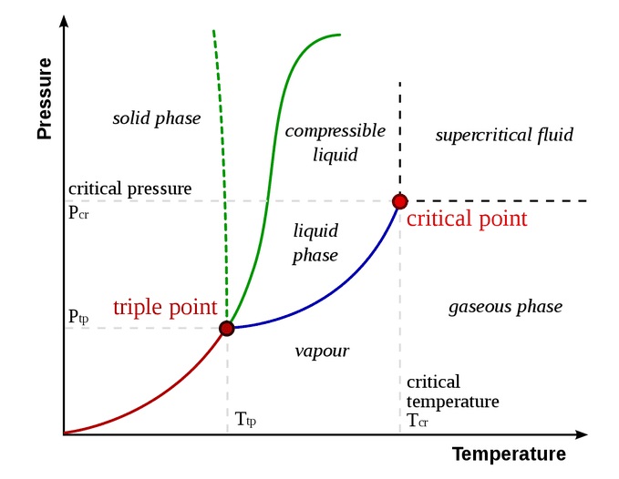
Part 11.4.7: Relative Humidity
The relative humidity $ {\displaystyle (RH} $ or $ {\displaystyle \phi )} $ of an air-water mixture is defined as the ratio of the partial pressure of water vapor $ {\displaystyle (p_{H_{2}O})} $ in the mixture to the equilibrium vapor pressure of water $ {\displaystyle (p_{H_{2}O}^{*})} $ over a flat surface of pure water at a given temperature:
$$ {\displaystyle \phi ={p_{H_{2}O} \over p_{H_{2}O}^{*}}} $$In other words, relative humidity is the ratio of how much water vapor is in the air and how much water vapor the air could potentially contain at a given temperature. It varies with the temperature of the air: colder air can hold less vapour. So changing the temperature of air can change the relative humidity, even when the absolute humidity remains constant.
Chilling air increases the relative humidity, and can cause the water vapor to condense (if the relative humidity rises over 100%, the dew point). Likewise, warming air decreases the relative humidity. Warming some air containing a fog may cause that fog to evaporate, as the air between the water droplets becomes more able to hold water vapour.
Relative humidity is normally expressed as a percentage; a higher percentage means that the air–water mixture is more humid. At 100% relative humidity, the air is saturated and is at its dew point. In the absence of a foreign body on which droplets or crystals can nucleate, the relative humidity can exceed 100%, in which case the air is said to be supersaturated. Introduction of some particles or a surface to a body of air above 100% relative humidity will allow condensation or ice to form on those nuclei.
Relative humidity is an important metric used in weather forecasts and reports, as it is an indicator of the likelihood of precipitation, dew, or fog. In hot summer weather, a rise in relative humidity increases the apparent temperature to humans.
Part 11.4.8: The Dew Point of Water
The dew point is the temperature to which air must be cooled to become saturated with water vapor, assuming constant air pressure and water content. When cooled below the dew point, the capacity to hold moisture is reduced and airborne water vapor will condense to form water droplets. When this occurs via contact with a colder surface, water droplets will form on that surface. In normal conditions, the dew point temperature will not be greater than the air temperature, since relative humidity typically does not exceed 100%.
In technical terms, the dew point is the temperature at which the water vapor in a sample of air at constant barometric pressure condenses into liquid water at the same rate at which it evaporates. At temperatures below the dew point, the rate of condensation will be greater than that of evaporation, forming more liquid water. The condensed water is called dew when it forms on a solid surface, or frost if it freezes. In the air, the condensed water is called either fog or a cloud, depending on its altitude when it forms. If the temperature is below the dew point, and no dew or fog forms, the vapor is called supersaturated. This can happen if there are not enough particles in the air to act as condensation nuclei.
The dew point depends on how much water vapor the air contains. If the air is very dry, the dew point is low and surfaces must be much cooler than the air for condensation to occur. If the air is very humid and contains a high density of water molecules, the dew point is high and condensation can occur on surfaces that are only a few degrees cooler than the air.
A high relative humidity implies that the dew point is close to the current air temperature. A relative humidity of 100% indicates the dew point is equal to the current temperature and that the air is maximally saturated with water. When the moisture content remains constant and temperature increases, relative humidity decreases, but the dew point remains constant.
Part 11.4.9: The Clausius–Clapeyron relation
The Clausius–Clapeyron relation specifies the temperature dependence of pressure, most importantly vapor pressure, at a discontinuous phase transition between two phases of matter of a single constituent. Its relevance to meteorology and climatology is the increase of the water-holding capacity of the atmosphere by about 7% for every 1 °C (1.8 °F) rise in temperature.
On a pressure–temperature $ {\displaystyle (P–T)} $ diagram, the line separating the two phases is known as the coexistence curve. The Clapeyron relation gives the slope of the tangents to this curve. Mathematically,
$$ {\displaystyle {\frac {\mathrm {d} P}{\mathrm {d} T}}={\frac {L}{T\,\Delta v}}={\frac {\Delta s}{\Delta v}},} $$where $ {\displaystyle \mathrm {d} P/\mathrm {d} T} $ is the slope of the tangent to the coexistence curve at any point, $ {\displaystyle L} $ is the specific latent heat, $ {\displaystyle T} $ is the temperature, $ {\displaystyle \Delta v} $ is the specific volume change of the phase transition, and $ {\displaystyle \Delta s} $ is the specific entropy change of the phase transition. The Clausius–Clapeyron equation:
$$ {\displaystyle {\frac {\mathrm {d} P}{\mathrm {d} T}}={\frac {PL}{T^{2}R}}} $$expresses this in a more convenient form just in terms of the latent heat, for moderate temperatures and pressures.
Derivation from state postulate
Using the state postulate and taking the specific entropy $ {\displaystyle s} $ for a homogeneous substance to be a function of specific volume $ {\displaystyle v} $ and temperature $ {\displaystyle T} $ .
$$ {\displaystyle \mathrm {d} s=\left({\frac {\partial s}{\partial v}}\right)_{T}\,\mathrm {d} v+\left({\frac {\partial s}{\partial T}}\right)_{v}\,\mathrm {d} T.} $$The Clausius–Clapeyron relation characterizes behavior of a closed system during a phase change at constant temperature and pressure. Therefore:
$$ {\displaystyle \mathrm {d} s=\left({\frac {\partial s}{\partial v}}\right)_{T}\,\mathrm {d} v.} $$Using the appropriate Maxwell relation gives:
$$ {\displaystyle \mathrm {d} s=\left({\frac {\partial P}{\partial T}}\right)_{v}\,\mathrm {d} v} $$where $ {\displaystyle P} $ is the pressure. Since pressure and temperature are constant, the derivative of pressure with respect to temperature does not change. Therefore, the partial derivative of specific entropy may be changed into a total derivative:
$$ {\displaystyle \mathrm {d} s={\frac {\mathrm {d} P}{\mathrm {d} T}}\,\mathrm {d} v} $$And the total derivative of pressure with respect to temperature may be factored out when integrating from an initial phase $ {\displaystyle \alpha } $ to a final phase $ {\displaystyle \beta } $ to obtain:
$$ {\displaystyle {\frac {\mathrm {d} P}{\mathrm {d} T}}={\frac {\Delta s}{\Delta v}}} $$where $ {\displaystyle \Delta s\equiv s_{\beta }-s_{\alpha }} $ and $ {\displaystyle \Delta v\equiv v_{\beta }-v_{\alpha }} $ are respectively the change in specific entropy and specific volume. Given that a phase change is an internally reversible process, and that our system is closed, the first law of thermodynamics holds:
$$ {\displaystyle \mathrm {d} u=\delta q+\delta w=T\;\mathrm {d} s-P\;\mathrm {d} v} $$where $ {\displaystyle u} $ is the internal energy of the system. Given constant pressure and temperature (during a phase change) and the definition of specific enthalpy $ {\displaystyle h} $ , we obtain:
$$ {\displaystyle \mathrm {d} h=T\;\mathrm {d} s+v\;\mathrm {d} P} $$ $$ {\displaystyle \mathrm {d} h=T\;\mathrm {d} s} $$ $$ {\displaystyle \mathrm {d} s={\frac {\mathrm {d} h}{T}}} $$Given constant pressure and temperature (during a phase change), we obtain:
$$ {\displaystyle \Delta s={\frac {\Delta h}{T}}} $$Substituting the definition of specific latent heat $ {\displaystyle L=\Delta h} $ gives:
$$ {\displaystyle \Delta s={\frac {L}{T}}} $$Substituting this result into the pressure derivative given above $ {\displaystyle \mathrm {d} P/\mathrm {d} T=\Delta s/\Delta v} $ we obtain:
$$ {\displaystyle {\frac {\mathrm {d} P}{\mathrm {d} T}}={\frac {L}{T\,\Delta v}}.} $$This result (also known as the Clapeyron equation) equates the slope $ {\displaystyle \mathrm {d} P/\mathrm {d} T} $ of the coexistence curve $ {\displaystyle P(T)} $ to the function $ {\displaystyle L/(T\,\Delta v)} $ of the specific latent heat $ {\displaystyle L} $ , the temperature $ {\displaystyle T} $ , and the change in specific volume $ {\displaystyle \Delta v} $ instead of the specific, corresponding molar values may also be used.
Part 11.5: Electrical Properties
Part 11.5.1: Electric Conductivity
Pure water containing no exogenous (non-$ {{H}_2}O $ ) ions is an excellent electronic insulator, but not even "deionized" water is completely free of ions. Water undergoes autoionization in the liquid state when two water molecules form one hydroxide anion $ (O{H}^−) $ and one hydronium cation $ ({{H}_3}{O}^+) $ .
Because of autoionization, at ambient temperatures pure liquid water has a similar intrinsic charge carrier concentration to the semiconductor germanium and an intrinsic charge carrier concentration three orders of magnitude greater than the semiconductor silicon, hence, based on charge carrier concentration, water can not be considered to be a completely dielectric material or electrical insulator but to be a limited conductor of ionic charge.
Because water is such a good solvent, it almost always has some solute dissolved in it, often a salt. If water has even a tiny amount of such an impurity, then the ions can carry charges, allowing the water to conduct electricity far more readily.
The theoretical maximum electrical resistivity for water is approximately 182 kΩ·m at 25 °C. This figure agrees well with what is typically seen on reverse osmosis, ultra-filtered and deionized ultra-pure water systems. A salt or acid contaminant level exceeding even 100 parts per trillion (ppt) in otherwise ultra-pure water begins to noticeably lower its resistivity by up to several kΩ·m.
In pure water, sensitive equipment can detect a very slight electrical conductivity of 0.05501 ± 0.0001 μS/cm at 25.00 °C. Water can also be electrolyzed into oxygen and hydrogen gases but in the absence of dissolved ions this is a very slow process, as very little current is conducted. In ice, the primary charge carriers are protons. Ice was previously thought to have a small but measurable conductivity of $ {1 × {10}^{−10} S/cm } $ , but this conductivity is now thought to be almost entirely from surface defects, and without those, ice is an insulator with an immeasurably small conductivity.
Part 11.5.2: Dipole Moment
The dipole moment arises because oxygen is more electronegative than hydrogen; the oxygen pulls in the shared electrons and increases the electron density around itself.
The dipole moment of water is $ {\displaystyle \mathbf {1.85 D} } $ or $ {\displaystyle \mathbf{ 6.17 x 10^{-30} C⋅m}} $ .
Part 11.5.3: Permittivity of Water
The relative permittivity is the permittivity of a material expressed as a ratio with the electric permittivity of a vacuum. A dielectric is an insulating material, and the dielectric constant of an insulator measures the ability of the insulator to store electric energy in an electrical field.
If a dielectric material is a linear dielectric, then electric susceptibility is defined as the constant of proportionality (which may be a matrix) relating an electric field $ {\displaystyle \mathbf {E}} $ to the induced dielectric polarization density $ {\displaystyle \mathbf {P}} $ such that:
$$ {\displaystyle \mathbf {P} =\varepsilon _{0}\chi _{\text{e}}{\mathbf {E} },} $$Where:
$ {\displaystyle \mathbf {P}} $ is the polarization density;
$ {\displaystyle \varepsilon _{0}} $ is the electric permittivity of free space;
$ {\displaystyle \chi _{\text{e}}} $ is the electric susceptibility;
$ {\displaystyle \mathbf {E}} $ is the electric field strength;
In materials where susceptibility is anisotropic (different depending on direction), susceptibility is represented as a matrix known as the susceptibility tensor. Many linear dielectrics are isotropic, but it is possible nevertheless for a material to display behavior that is both linear and anisotropic, or for a material to be non-linear but isotropic. Anisotropic but linear susceptibility is common in many crystals.
Part 11.6: Moleacular Structure of Water
A single water molecule can participate in a maximum of four hydrogen bonds because it can accept two bonds using the lone pairs on oxygen and donate two hydrogen atoms. Other molecules like hydrogen fluoride, ammonia, and methanol can also form hydrogen bonds. However, they do not show anomalous thermodynamic, kinetic, or structural properties like those observed in water because none of them can form four hydrogen bonds: either they cannot donate or accept hydrogen atoms, or there are steric effects in bulky residues.
In water, intermolecular tetrahedral structures form due to the four hydrogen bonds, thereby forming an open structure and a three-dimensional bonding network, resulting in the anomalous decrease in density when cooled below 4 °C. This repeated, constantly reorganizing unit defines a three-dimensional network extending throughout the liquid. This view is based upon neutron scattering studies and computer simulations, and it makes sense in the light of the unambiguously tetrahedral arrangement of water molecules in ice structures.
Molecular Structure
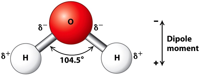
Tetrahedral Structure
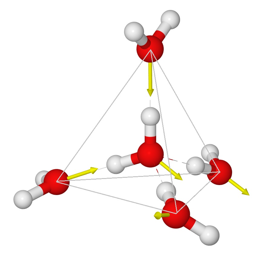
The repulsive effects of the two lone pairs on the oxygen atom cause water to have a bent molecular structure, allowing it to be polar. The hydrogen–oxygen–hydrogen angle is 104.45°, which is less than the 109.47° for ideal $ {\displaystyle sp^3} $ hybridization.
The valence bond theory explanation is that the oxygen atom's lone pairs are physically larger and therefore take up more space than the oxygen atom's bonds to the hydrogen atoms.
The molecular orbital theory explanation (Bent's rule) is that lowering the energy of the oxygen atom's nonbonding hybrid orbitals (by assigning them more $ {\displaystyle s} $ character and less $ {\displaystyle p} $ character) and correspondingly raising the energy of the oxygen atom's hybrid orbitals bonded to the hydrogen atoms (by assigning them more $ {\displaystyle p} $ character and less $ {\displaystyle s} $ character) has the net effect of lowering the energy of the occupied molecular orbitals because the energy of the oxygen atom's nonbonding hybrid orbitals contributes completely to the energy of the oxygen atom's lone pairs while the energy of the oxygen atom's other two hybrid orbitals contributes only partially to the energy of the bonding orbitals (the remainder of the contribution coming from the hydrogen atoms' $ {\displaystyle 1s} $ orbitals).
Part 11.7: Chemical Properties
Self-Ionization: The self-ionization of water was first proposed in 1884 by Svante Arrhenius as part of the theory of ionic dissociation which he proposed to explain the conductivity of electrolytes including water. Arrhenius wrote the self-ionization as:
$$ {\displaystyle {{H_2}O <=> H^+ + OH^-}} $$ .At that time, nothing was yet known of atomic structure or subatomic particles, so he had no reason to consider the formation of an $ {\displaystyle {H^+}} $ ion from a hydrogen atom on electrolysis as any less likely than, say, the formation of a $ {\displaystyle {Na^+}} $ ion from a sodium atom.
In 1923 Johannes Nicolaus Brønsted and Martin Lowry proposed that the self-ionization of water actually involves two water molecules:
$$ {\displaystyle {{H_2}O + {H_2}O <=> {H_3}O^+ + OH^-}} $$ .By this time the electron and the nucleus had been discovered and Rutherford had shown that a nucleus is very much smaller than an atom. This would include a bare ion $ {\displaystyle {H^+}} $ which would correspond to a proton with zero electrons. Brønsted and Lowry proposed that this ion does not exist free in solution, but always attaches itself to a water (or other solvent) molecule to form the hydronium ion $ {\displaystyle {{H_3}O^+}} $ .
Later spectroscopic evidence has shown that many protons are actually hydrated by more than one water molecule. The most descriptive notation for the hydrated ion is $ {\displaystyle {H^+(aq)}} $ , where aq (for aqueous) indicates an indefinite or variable number of water molecules. However the notations $ {\displaystyle {H^+}} $ and $ {\displaystyle {{H_3}O^+}} $ are still also used extensively because of their historical importance. This document mostly represents the hydrated proton as $ {\displaystyle {{H_3}O^+}} $ , corresponding to hydration by a single water molecule.
Chemically pure water has an electrical conductivity of 0.055 μS/cm. According to the theories of Svante Arrhenius, this must be due to the presence of ions. The ions are produced by the water self-ionization reaction, which applies to pure water and any aqueous solution:
$$ {\displaystyle {{H_2}O + {H_2}O <=> {H_3}O^+ + OH^-}} $$Expressed with chemical activities $ {\displaystyle a} $ , instead of concentrations, the thermodynamic equilibrium constant for the water ionization reaction is:
$$ {\displaystyle K_{\rm {eq}}={\frac {a_{\rm {H_{3}O^{+}}}\cdot a_{\rm {OH^{-}}}}{a_{\rm {H_{2}O}}^{2}}}} $$Which is numerically equal to the more traditional thermodynamic equilibrium constant written as:
$$ {\displaystyle K_{\rm {eq}}={\frac {a_{\rm {H^{+}}}\cdot a_{\rm {OH^{-}}}}{a_{\rm {H_{2}O}}}}} $$Under the assumption that the sum of the chemical potentials of $ {\displaystyle H^+} $ and $ {\displaystyle {H_3}O+} $ is formally equal to twice the chemical potential of $ {\displaystyle {H_2}O} $ at the same temperature and pressure.
Because most acid–base solutions are typically very dilute, the activity of water is generally approximated as being equal to unity, which allows the ionic product of water to be expressed as:
$$ {\displaystyle K_{\rm {eq}}\approx a_{\rm {H_{3}O^{+}}}\cdot a_{\rm {OH^{-}}}} $$In dilute aqueous solutions, the activities of solutes (dissolved species such as ions) are approximately equal to their concentrations. Thus, the ionization constant, dissociation constant, self-ionization constant, water ion-product constant or ionic product of water, symbolized by $ {\displaystyle K_w} $ , may be given by:
$$ {\displaystyle K_{\rm {w}}=[{\rm {H_{3}O^{+}}}][{\rm {OH^{-}}}]} $$where $ {\displaystyle {[H_3}O^+]} $ is the molarity (≈ molar concentration) of hydrogen or hydronium ion, and $ {\displaystyle {[OH^-]}} $ is the concentration of hydroxide ion. When the equilibrium constant is written as a product of concentrations (as opposed to activities) it is necessary to make corrections to the value of $ {\displaystyle K_{\rm {w}}} $ depending on ionic strength and other factors.
At 24.87 °C and zero ionic strength, $ {\displaystyle K_{\rm {w}}} $ is equal to $ {\displaystyle {1.0×10^{−14}}} $ . Note that as with all equilibrium constants, the result is dimensionless because the concentration is in fact a concentration relative to the standard state, which for $ {\displaystyle H^+ } $ and $ {\displaystyle OH^-} $ are both defined to be 1 molal (or nearly 1 molar).
For many practical purposes, the molal (mol solute/kg water) and molar (mol solute/L solution) concentrations can be considered as nearly equal at ambient temperature and pressure if the solution density remains close to one. The main advantage of the molal concentration unit (mol/kg water) is to result in stable and robust concentration values which are independent of the solution density and volume changes (density depending on the water salinity (ionic strength), temperature and pressure); therefore, molality is the preferred unit used in thermodynamic calculations or in precise or less-usual conditions, e.g., for seawater with a density significantly different from that of pure water, or at elevated temperatures, like those prevailing in thermal power plants.
Part 11.8: Surface Tension
Surface tension is the tendency of liquid surfaces at rest to shrink into the minimum surface area possible. Surface tension is what allows objects with a higher density than water such as razor blades to float on a water surface without becoming even partly submerged. At liquid–saturated air interfaces, surface tension results from the greater attraction of liquid molecules to each other (due to cohesion) than to the molecules in the water vapour (due to adhesion).
There are two primary mechanisms in play. One is an inward force on the surface molecules causing the liquid to contract. Second is a tangential force parallel to the surface of the liquid. This tangential force is generally referred to as the surface tension. The net effect is the liquid behaves as if its surface were covered with a stretched elastic membrane.
Because of the relatively high attraction of water molecules to each other through a web of hydrogen bonds and the fact that the water moleacule is highly polar, the water moleacule has a higher surface tension (72.8 millinewtons per meter at 20 °C) than most other liquids. Surface tension is an important factor in the stability of water droplets in the atmosphere.
Surface tension has the dimension of force per unit length, or of energy per unit area. The two are equivalent, but when referring to energy per unit of area, it is common to use the term surface energy.
Due to the cohesive forces, a molecule located away from the surface is pulled equally in every direction by neighbouring liquid molecules, resulting in a net force of zero. The molecules at the surface do not have the same molecules on all sides of them and therefore are pulled inward. This creates some internal pressure and forces liquid surfaces to contract to the minimum area.
There is also a tension parallel to the surface at the water-air interface which will resist an external force, due to the cohesive nature of water molecules.
The forces of attraction acting between water molecules are called cohesive forces, while those acting between molecules of different types are called adhesive forces. The balance between the cohesion of the water and its adhesion to the air moleacules surounding the water droplet determines the contact angle and the spherical shape of the water droplet.
Surface tension is responsible for the shape of water droplets. Although easily deformed, droplets of water tend to be pulled into a spherical shape by the imbalance in cohesive forces of the surface layer. In the absence of other forces, drops of water would be approximately spherical. The spherical shape minimizes the necessary "wall tension" of the surface layer.
Part 11.8.1: Surface Tension In terms of energy:
Another way to view surface tension is in terms of energy. A molecule in contact with a neighbor is in a lower state of energy than if it were alone. The interior molecules have as many neighbors as they can possibly have, but the boundary molecules are missing neighbors (compared to interior molecules) and therefore have a higher energy. For the liquid to minimize its energy state, the number of higher energy boundary molecules must be minimized. The minimized number of boundary molecules results in a minimal surface area. As a result of surface area minimization, a surface will assume the smoothest shape it can. Since any curvature in the surface shape results in greater area, a higher energy will also result.
Surface tension $ {\displaystyle \gamma } $ of a liquid is the ratio of the change in the energy of the liquid to the change in the surface area of the liquid (that led to the change in energy). This can be easily related to the definition in terms of force: if $ {\displaystyle F } $ is the force required to stop the side from starting to slide, then this is also the force that would keep the side in the state of sliding at a constant speed (by Newton's Second Law). But if the side is moving to the right (in the direction the force is applied), then the surface area of the stretched liquid is increasing while the applied force is doing work on the liquid. This means that increasing the surface area increases the energy of the film.
The work done by the force $ {\displaystyle F } $ in moving the side by distance $ {\displaystyle \delta x } $ is $ {\displaystyle W = F \delta x } $ ; at the same time the total area of the film increases by $ {\displaystyle \delta A = 2 L \delta x } $ . Thus, multiplying both the numerator and the denominator of $ {\displaystyle \gamma = {1/2} F/L } $ by $ {\displaystyle \delta x } $ , we get:
$$ {\displaystyle \gamma ={\frac {F}{2L}}={\frac {F\Delta x}{2L\Delta x}}={\frac {W}{\Delta A}}.} $$This work $ {\displaystyle W } $ is interpreted as being stored as potential energy. Consequently, surface tension can be also measured in SI system as joules per square meter and in the cgs system as ergs per $ {\displaystyle {cm}^2. } $ Since mechanical systems try to find a state of minimum potential energy, a free droplet of liquid naturally assumes a spherical shape, which has the minimum surface area for a given volume.
Part 11.8.2: Surface Curvature and Pressure
If no force acts normal to a tensioned surface, the surface must remain flat. But if the pressure on one side of the surface differs from pressure on the other side, the pressure difference times surface area results in a normal force. In order for the surface tension forces to cancel the force due to pressure, the surface must be curved. Surface curvature of a tiny patch of surface leads to a net component of surface tension forces acting normal to the center of the patch. When all the forces are balanced, the resulting equation is known as the Young–Laplace equation:
$$ {\displaystyle \Delta p=\gamma \left({\frac {1}{R_{x}}}+{\frac {1}{R_{y}}}\right)} $$Where:
- $ {\displaystyle \delta p } $ is the pressure difference, known as the Laplace pressure.
- $ {\displaystyle \gamma } $ is the surface tension
- $ {\displaystyle R x } $ and $ {\displaystyle R y } $ are radii of curvature in each of the axes that are parallel to the surface
The quantity in parentheses on the right hand side is in fact (twice) the mean curvature of the surface. Solutions to this equation determine the shape of water droplets. The pressure of a water droplet increases with decreasing radius. For large drops the effect is subtle, but the pressure difference becomes enormous when the drop sizes approach the molecular size.
Water molecules want to cling to each other. At the surface, however, there are fewer water molecules to cling to since there is air above (thus, no water molecules). This results in a stronger bond between those molecules that actually do come in contact with one another, and a layer of strongly bonded water. This surface layer (held together by surface tension) creates a considerable barrier between the atmosphere and the water. In fact, other than mercury, water has the greatest surface tension of any liquid.
Within a body of a liquid, a molecule will not experience a net force because the forces by the neighboring molecules all cancel out. However for a molecule on the surface of the liquid, there will be a net inward force since there will be no attractive force acting from above. This inward net force causes the molecules on the surface to contract and to resist being stretched or broken. Thus the surface is under tension.
Part 11.9: Electromagnetic Interaction
Solar Radiation Absorption Since the primary purpose of this document is the description of the electromagnetic interaction of negative-ions with the atmospheric water moleacules in the troposphere we will be mainly discussing the absorption of electromagnetic radiation by water molecules, in the gaseous state. In the gaseous state water has three types of transition that can give rise to absorption of electromagnetic radiation: 1. Rotational transitions:: Transitions in which the molecule gains a quantum of rotational energy. Atmospheric water vapour at ambient temperature and pressure gives rise to absorption in the far-infrared region of the spectrum, from about (50 μm) to longer wavelengths towards the microwave region. The water molecule is an asymmetric top, that is, it has three independent moments of inertia. Because of the low symmetry of the molecule, a large number of transitions can be observed in the far infrared region of the spectrum. Measurements of microwave spectra have provided a very precise value for the O−H bond length, 95.84 ± 0.05 pm and H−O−H bond angle, 104.5 ± 0.3° 2. Vibrational transitions: Transitions in which a molecule gains a quantum of vibrational energy. The fundamental transitions give rise to absorption in the mid-infrared in the regions around $ {\displaystyle {1650 {cm}^{−1}}} $ (μ band, 6 μm) and $ {\displaystyle {3500 {cm}^{−1}}} $ (so-called X band, 2.9 μm) The water molecule has three fundamental molecular vibrations. The O-H stretching vibrations give rise to absorption bands with band origins at 3657 cm−1 (ν1, 2.734 μm) and 3756 cm−1 (ν3, 2.662 μm) in the gas phase. The asymmetric stretching vibration, of B2 symmetry in the point group C2v is a normal vibration. The H-O-H bending mode origin is at 1595 cm−1 (ν2, 6.269 μm). Both symmetric stretching and bending vibrations have A1 symmetry, but the frequency difference between them is so large that mixing is effectively zero. In the gas phase all three bands show extensive rotational fine structure. In the Near-infrared spectrum ν3 has a series of overtones at wavenumbers somewhat less than n·ν3, n=2,3,4,5... Combination bands, such as ν2 + ν3 are also easily observed in the near-infrared region. The presence of water vapor in the atmosphere is important for atmospheric chemistry especially as the infrared and near infrared spectra are easy to observe. Standard (atmospheric optical) codes are assigned to absorption bands as follows. 0.718 μm (visible): α, 0.810 μm: μ, 0.935 μm: ρστ, 1.13 μm: φ, 1.38 μm: ψ, 1.88 μm: Ω, 2.68 μm: X. The gaps between the bands define the infrared window in the Earth's atmosphere. In reality, vibrations of molecules in the gaseous state are accompanied by rotational transitions, giving rise to a vibration-rotation spectrum. Furthermore, vibrational overtones and combination bands occur in the near-infrared region. The HITRAN spectroscopy database lists more than 37,000 spectral lines for gaseous $ {\displaystyle {H_2}0^{16}} $ , ranging from the microwave region to the visible spectrum. In liquid water the rotational transitions are effectively quenched, but absorption bands are affected by hydrogen bonding. In crystalline ice the vibrational spectrum is also affected by hydrogen bonding and there are lattice vibrations causing absorption in the far-infrared. Electronic transitions of gaseous molecules will show both vibrational and rotational fine structure. 3. Electronic Transitions: Transitions in which a molecule is promoted to an excited electronic state. The lowest energy transition of this type is in the vacuum ultraviolet region. For water vapor the bands have been assigned as follows. At least some of these transitions result in photo-dissociation of water into $ {\displaystyle {H^+}} $ and $ {\displaystyle {0H^-}} $ . Among them the best known is that at 166.5 nm. The infrared spectrum of liquid water is dominated by the intense absorption due to the fundamental $ {\displaystyle {O-H}} $ stretching vibrations. Because of the high intensity, very short path lengths, usually less than 50 μm, are needed to record the spectra of aqueous solutions. There is no rotational fine structure, but the absorption bands are broader than might be expected, because of hydrogen bonding. Peak maxima for liquid water are observed at 3450 $ {\displaystyle {cm^{-1}}} $ (2.898 μm), 3615 $ {\displaystyle {cm^{-1}}} $ (2.766 μm) and 1640 $ {\displaystyle {cm^{-1}}} $ (6.097 μm). Direct measurement of the infrared spectra of aqueous solutions requires that the cuvette windows be made of substances such as calcium fluoride which are water-insoluble. Water vapor is the most important greenhouse gas in the Earth's atmosphere, responsible for more than 70% of the known absorption of incoming sunlight, particularly in the infrared region, and about 90% of the atmospheric absorption of thermal radiation by the Earth known as the greenhouse effect. In the atmospheric window between approximately 8000 and 14000 nm, the far-infrared spectrum, water absorption is weak. This window allows most of the thermal radiation in this band to be radiated out to space directly from the Earth's surface. As well as absorbing radiation, water vapour emits radiation in all directions, according to the Black Body Emission curve for its current temperature overlaid on the water absorption spectrum. Much of this energy will be recaptured by other water molecules, but at higher altitudes, radiation sent towards space is less likely to be recaptured, as there is less water available to recapture radiation of water-specific absorbing wavelengths. By the top of the troposphere, about 12 km above sea level, most water vapor condenses to liquid water or ice as it releases its heat of vapourization. Once changed state, liquid water and ice fall away to lower altitudes. This will be balanced by incoming water vapour rising via convection currents. Liquid water and ice emit radiation at a higher rate than water vapour. Water at the top of the troposphere, particularly in liquid and solid states, cools as it emits net photons to space. Neighboring gas molecules other than water (e.g. Nitrogen) are cooled by passing their energy kinetically to the water. This is why temperatures at the top of the troposphere (known as the tropopause) are about -50 degrees Celsius. An Aerosol is defined as a suspension system of solid or liquid particles in a gas. An aerosol includes both the particles and the suspending gas, which in the case of atmospherics is air. Meteorologists usually refer them as particulate matter $ {\displaystyle PM_{2.5} } $ or $ {\displaystyle PM_{10} } $ , depending on their size. The key aerosols, to be discussed in this document will be: negative ions and electrified water droplets. In the meterology literature the key aerosol groups include sulfates, organic carbon, black carbon, nitrates, mineral dust, and sea salt. The predominent aerosol in cloud formation is sea salt. These earosol clump together in the troposphere to form a complex mixture. There are several measures of aerosol concentration. Environmental science and environmental health often use the mass concentration (M), defined as the mass of particulate matter per unit volume, in units such as $ {\displaystyle {\mu g/m^3}} $ . Also commonly used is the number concentration (N), the number of particles per unit volume. Particle size has a major influence on particle properties, and the aerosol particle radius or diameter is a key property used to characterise aerosols. Aerosols vary in their dispersity. A monodisperse aerosol, producible in the laboratory, contains particles of uniform size. Most aerosols, however, as polydisperse colloidal systems, exhibit a range of particle sizes. Liquid droplets are almost always nearly spherical, but scientists use an equivalent diameter to characterize the properties of various shapes of solid particles, some very irregular. The equivalent diameter is the diameter of a spherical particle with the same value of some physical property as the irregular particle. The equivalent volume diameter is defined as the diameter of a sphere of the same volume as that of the irregular particle. For a mono-disperse aerosol, a single number—the particle diameter—suffices to describe the size of the particles. However, more complicated particle-size distributions describe the sizes of the particles in a poly-disperse aerosol. This distribution defines the relative amounts of particles, sorted according to size. One approach to defining the particle size distribution uses a list of the sizes of every particle in a sample. However, this approach proves tedious to ascertain in aerosols with millions of particles and awkward to use. Another approach splits the size range into intervals and finds the number (or proportion) of particles in each interval. These data can be presented in a histogram with the area of each bar representing the proportion of particles in that size bin, usually normalised by dividing the number of particles in a bin by the width of the interval so that the area of each bar is proportionate to the number of particles in the size range that it represents. If the width of the bins tends to zero, the frequency function is: Where: $ {\displaystyle d_{p}} $ is the diameter of the particles $ {\displaystyle \mathrm {d} f} $ is the fraction of particles having diameters between $ {\displaystyle d_{p}} $ and $ {\displaystyle d_{p}} $ $ + {\displaystyle \mathrm {d} d_{p}} $ $ {\displaystyle f(d_{p})} $ is a characteristic linear dimension in meters Therefore, the area under the frequency curve between two sizes $ {\displaystyle a} $ and $ {\displaystyle b} $ represents the total fraction of the particles in that size range: It can also be formulated in terms of the total number density $ N $ : Assuming spherical aerosol particles, the aerosol surface area per unit volume $ (S) $ is given by the second moment: And the third moment gives the total volume concentration $ (V) $ of the particles: The particle size distribution can be approximated. The normal distribution usually does not suitably describe particle size distributions in aerosols because of the skewness associated with a long tail of larger particles. Also for a quantity that varies over a large range, as many aerosol sizes do, the width of the distribution implies negative particles sizes, which is not physically realistic. A more widely chosen log-normal distribution gives the number frequency as: Where: $ {\displaystyle d_{p}} $ is the diameter of the particles $ {\displaystyle \mathrm {d} f} $ is the fraction of particles having diameters between $ {\displaystyle d_{p}} $ and $ {\displaystyle d_{p}} $ $ + {\displaystyle \mathrm {d} d_{p}} $ $ {\displaystyle f(d_{p})} $ is a characteristic linear dimension in meters $ {\displaystyle \sigma } $ is the standard deviation of the size distribution and $ {\displaystyle {\bar {d_{p}}}} $ is the arithmetic mean diameter. The log-normal distribution has no negative values, can cover a wide range of values, and fits many observed size distributions reasonably well. Other distributions sometimes used to characterise particle size include: the Rosin-Rammler distribution, applied to coarsely dispersed dusts and sprays; the Nukiyama–Tanasawa distribution, for sprays of extremely broad size ranges; the power function distribution, occasionally applied to atmospheric aerosols; the exponential distribution, applied to powdered materials; and for cloud droplets, the Khrgian–Mazin distribution. For low values of the Reynolds number $ {\displaystyle (<1) } $ , true for most aerosol motion, Stokes' law describes the force of resistance on a solid spherical particle in a fluid. However, Stokes' law is only valid when the velocity of the gas at the surface of the particle is zero. For small particles $ {\displaystyle (<1 \mu m)} $ that characterize aerosols, however, this assumption fails. To account for this failure, one can introduce the Cunningham correction factor, always greater than 1. Including this factor, one finds the relation between the resisting force on a particle and its velocity: Where: $ {\displaystyle F_{D}} $ is the resisting force on a spherical particle $ {\displaystyle \eta } $ is the dynamic viscosity of the gas $ {\displaystyle V} $ is the particle velocity $ {\displaystyle C_{c}} $ is the Cunningham correction factor. This allows us to calculate the terminal velocity of a particle undergoing gravitational settling in still air. Neglecting buoyancy effects, we find: Where: $ {\displaystyle V_{TS}} $ is the terminal settling velocity of the particle. The terminal velocity can also be derived for other kinds of forces. If Stokes' law holds, then the resistance to motion is directly proportional to speed. The constant of proportionality is the mechanical mobility of a particle: A particle traveling at any reasonable initial velocity approaches its terminal velocity exponentially with an e-folding time equal to the relaxation time: Where: $ {\displaystyle V(t)} $ is the particle speed at time t $ {\displaystyle V_{f}} $ is the final particle speed $ {\displaystyle V_{0}} $ is the initial particle speed To account for the effect of the shape of non-spherical particles, a correction factor known as the dynamic shape factor is applied to Stokes' law. It is defined as the ratio of the resistive force of the irregular particle to that of a spherical particle with the same volume and velocity: Where: $ {\displaystyle \chi } $ is the dynamic shape factor The previous discussion focused on single aerosol particles. In contrast, aerosol dynamics explains the evolution of complete aerosol populations. The concentrations of particles will change over time as a result of many processes. External processes that move particles outside a volume of gas under study include diffusion, gravitational settling, and electric charges and other external forces that cause particle migration. A second set of processes internal to a given volume of gas include particle formation (nucleation), evaporation, chemical reaction, and coagulation. A differential equation called the Aerosol General Dynamic Equation characterizes the evolution of the number density of particles in an aerosol due to these processes. Change in time = Convective transport + brownian diffusion + gas-particle interactions + coagulation + migration by external forces Where: $ {\displaystyle n_{i}} $ is number density of particles of size category $ {\displaystyle i} $ $ {\displaystyle \mathbf {q} } $ is the particle velocity $ {\displaystyle D_{p}} $ is the particle Stokes-Einstein diffusivity $ {\displaystyle \mathbf {q} _{F}} $ is the particle velocity associated with an external force As particles and droplets in an aerosol collide with one another, they may undergo coalescence or aggregation. This process leads to a change in the aerosol particle-size distribution, with the mode increasing in diameter as total number of particles decreases. On occasion, particles may shatter apart into numerous smaller particles. Dynamics Regimes: The Knudsen number of the particle define three different dynamical regimes that govern the behaviour of an aerosol: Where: $ {\displaystyle K_{n} }$ is the Knudsen number $ {\displaystyle \lambda }$ is the mean free path of the suspending gas $ {\displaystyle d} $ is the diameter of the particle. For particles in the free molecular regime, $ {\displaystyle K_{n} >> 1 }$ ; particles small compared to the mean free path of the suspending gas. In this regime, particles interact with the suspending gas through a series of "ballistic" collisions with gas molecules. As such, they behave similarly to gas molecules, tending to follow streamlines and diffusing rapidly through Brownian motion. The mass flux equation in the free molecular regime is: Where: $ {\displaystyle a}$ is the particle radius, $ {\displaystyle P_{\infty }}$ and $ {\displaystyle P_A}$ are the pressures far from the droplet and at the surface of the droplet respectively $ {\displaystyle k_b}$ is the Boltzmann constant $ {\displaystyle T} $ is the temperature $ {\displaystyle C_A}$ is mean thermal velocity $ {\displaystyle \alpha }$ is mass accommodation coefficient The derivation of this equation assumes constant pressure and constant diffusion coefficient. Particles are in the continuum regime when $ {\displaystyle K_{n} << 1 }$ . In this regime, the particles are big compared to the mean free path of the suspending gas, meaning that the suspending gas acts as a continuous fluid flowing round the particle. The molecular flux in this regime is: Where $ {\displaystyle a}$ is the radius of the particle $ {\displaystyle A}$ , $ {\displaystyle M_A}$ is the molecular mass of the particle $ {\displaystyle A}$ , $ {\displaystyle D_{AB}}$ is the diffusion coefficient between particles $ {\displaystyle A}$ and $ {\displaystyle B}$ , $ {\displaystyle R}$ is the ideal gas constant, $ {\displaystyle T}$ is the temperature (in absolute units like kelvin), and $ {\displaystyle P_{A\infty}}$ and $ {\displaystyle P_{AS}}$ are the pressures at infinite and at the surface respectively. The transition regime contains all the particles in between the free molecular and continuum regimes or Kn ≈ 1. The forces experienced by a particle are a complex combination of interactions with individual gas molecules and macroscopic interactions. The semi-empirical equation describing mass flux is: where $ {\displaystyle I_{cont}}$ is the mass flux in the continuum regime. This formula is called the Fuchs-Sutugin interpolation formula. These equations do not take into account the heat release effect. Several types of atmospheric aerosol have a significant effect on Earth's climate: sea-salt, volcanic and desert dust, that originating from biogenic sources and human-made. Sea salt is the most prevelent atmospheric aerosol since it is part of the evaporation of ocean salt water. Volcanic aerosol forms in the stratosphere after an eruption as droplets of sulfuric acid that can prevail for up to two years, and reflect sunlight, lowering temperature. Desert dust, mineral particles blown to high altitudes, absorb heat and may be responsible for inhibiting storm cloud formation. Although all hydrometeors, solid and liquid, can be described as aerosols, a distinction is commonly made between such dispersions (i.e. clouds) containing activated drops and crystals, and aerosol particles. The atmosphere of Earth contains aerosols of various types and concentrations. Statistical physics is a branch of physics that evolved from a foundation of statistical mechanics, which uses methods of probability theory and statistics, and particularly the mathematical tools for dealing with large populations and approximations, in solving physical problems. It can describe a wide variety of fields with an inherently stochastic nature. Its applications include many problems in the fields of physics, biology, chemistry, neuroscience. Its main purpose is to clarify the properties of matter in aggregate, in terms of physical laws governing moleacular and atomic motion in the atmosphere. For the presentation in this document it will be used to introduce the theories of Turbulance and Vorticity Statistical Mechanics is used to develop the phenomenological results of thermodynamics from a probabilistic examination of the underlying microscopic systems. Historically, one of the first topics in physics where statistical methods were applied was the field of classical mechanics, which is concerned with the motion of particles or objects when subjected to a force. In our analysis of the microphysics of the atmosphere we need to consider the theories of thermodynamics within the context of classical mechanics as created by Newton, Lagrange and Hamilton. We must also include the appropriate elements of the theories of fluid mechanics and heat transfer. For these theories of mechanics, standard mathematical approaches have only been developed to solve a few, fairly simple mechanical models. In analytic mechanics the state of the mechanical system at a given time (the initial conditions), mathematically encoded at a phase point can lead to a set of differential equations which can be solved to predict the progression of the phase point into the future. The equations of motion carries the state forward in time. Using these concepts, the state at any other time in the future, can in principle be calculated. There is however a disconnect between these laws and everyday life experiences, as we do not find it necessary (nor even theoretically possible) to know exactly at a microscopic level the simultaneous positions and velocities of each molecule while carrying out processes at the human scale. Statistical mechanics atempts to fills this large gap between the laws of mechanics and the practical experience of incomplete knowledge, by adding some uncertainty about which state the system is in. Whereas ordinary mechanics only considers the behaviour of a single state, statistical mechanics introduces the statistical ensemble, which is a large collection of virtual, independent copies of the system in various states. The statistical ensemble is a probability distribution over all possible states of the system. In classical statistical mechanics, the ensemble is a probability distribution over phase points (as opposed to a single phase point in ordinary mechanics), usually represented as a distribution in a phase space with canonical coordinate axes. As is usual for probabilities, the ensemble can be interpreted in different ways: 1. An ensemble can be taken to represent the various possible states that a single system could be in. 2. The members of the ensemble can be understood as the states of the systems in experiments repeated on independent systems which have been prepared in a similar but imperfectly controlled manner (empirical probability), in the limit of an infinite number of trials. However the probability is interpreted, each state in the ensemble evolves over time according to the equation of motion. Thus, the ensemble itself (the probability distribution over states) also evolves, as the virtual systems in the ensemble continually leave one state and enter another. The ensemble evolution is given by the Liouville equation (classical mechanics) or the von Neumann equation (quantum mechanics). These equations are simply derived by the application of the mechanical equation of motion separately to each virtual system contained in the ensemble, with the probability of the virtual system being conserved over time as it evolves from state to state. One special, theoretical, class of ensemble is those ensembles that do not evolve over time. These ensembles are known as equilibrium ensembles and their condition is known as statistical equilibrium. Statistical equilibrium occurs if, for each state in the ensemble, the ensemble also contains all of its future and past states with probabilities equal to the probability of being in that state. The study of equilibrium ensembles of isolated systems is the focus of statistical thermodynamics. Non-equilibrium statistical mechanics addresses the more general case of ensembles that change over time, and/or ensembles of non-isolated systems. Unfortunately the atmosphere is always in a non-equilibrium state. Statistical Thermodynamics The primary goal of statistical thermodynamics is to derive the classical thermodynamics of materials in terms of the properties of their constituent particles and the interactions between them. In other words, statistical thermodynamics provides a connection between the macroscopic properties of materials in thermodynamic equilibrium, and the microscopic behaviours and motions occurring inside the material. Whereas statistical mechanics proper involves dynamics, here the attention is focussed on statistical equilibrium (steady state). Statistical equilibrium does not mean that the particles have stopped moving (mechanical equilibrium), rather, only that the ensemble is not evolving. Fundamental postulate A sufficient (but not necessary) condition for statistical equilibrium with an isolated system is that the probability distribution is a function only of conserved properties (total energy, total particle numbers, etc.). There are many different equilibrium ensembles that can be considered, and only some of them correspond to thermodynamics. Additional postulates are necessary to motivate why the ensemble for a given system should have one form or another. A common and simple approach is to take the equal a priori probability postulate. This postulate states that: For an isolated system with an exactly known energy and exactly known composition, the system can be found with equal probability in any microstate consistent with that knowledge. The equal a priori probability postulate therefore provides a motivation for the microcanonical ensemble described below. There are various arguments in favour of the equal a priori probability postulate: Ergodic hypothesis: An ergodic system is one that evolves over time to explore "all accessible" states: all those with the same energy and composition. In an ergodic system, the microcanonical ensemble is the only possible equilibrium ensemble with fixed energy. This approach has limited applicability, since most systems are not ergodic. Principle of indifference: In the absence of any further information, we can only assign equal probabilities to each compatible situation. Maximum information entropy: A more elaborate version of the principle of indifference states that the correct ensemble is the ensemble that is compatible with the known information and that has the largest Gibbs entropy (information entropy). Three Thermodynamic Ensembles There are three equilibrium ensembles with a simple form that can be defined for any isolated system bounded inside a finite volume. These are the most often discussed ensembles in statistical thermodynamics. In the macroscopic limit they all correspond to classical thermodynamics. 1. Microcanonical Ensemble Describes a system with a precisely given energy and fixed composition (precise number of particles). The microcanonical ensemble contains with equal probability each possible state that is consistent with that energy and composition. 2. Canonical Ensemble Describes a system of fixed composition that is in thermal equilibrium with a heat bath of a precise temperature. The canonical ensemble contains states of varying energy but identical composition; the different states in the ensemble are accorded different probabilities depending on their total energy. 3. Grand Canonical Ensemble Describes a system with non-fixed composition (uncertain particle numbers) that is in thermal and chemical equilibrium with a thermodynamic reservoir. The reservoir has a precise temperature, and precise chemical potentials for various types of particle. The grand canonical ensemble contains states of varying energy and varying numbers of particles; the different states in the ensemble are accorded different probabilities depending on their total energy and total particle numbers. For systems containing many particles (the thermodynamic limit), all three of the ensembles listed above tend to give identical behaviour. It is then simply a matter of mathematical convenience which ensemble is used. The Gibbs theorem about equivalence of ensembles was developed into the theory of concentration of measure phenomenon. In the study of atmospheric physics the Maxwell–Boltzmann distribution is the probability distribution which is most often used to study the distribution of Energy in the troposphere. It was first defined and used for describing particle speeds in idealized gases, where the particles move freely inside a stationary container without interacting with one another, except for very brief collisions in which they exchange energy and momentum with each other or with their thermal environment. The term "particle" in this context refers to gaseous particles only (atoms or molecules), and the system of particles is assumed to have reached thermodynamic equilibrium. The energies of such particles follow what is known as Maxwell–Boltzmann statistics, and the statistical distribution of speeds is derived by equating particle energies with kinetic energy. Mathematically, the Maxwell–Boltzmann distribution is the chi distribution with three degrees of freedom (the components of the velocity vector in Euclidean space), with a scale parameter measuring speeds in units proportional to the square root of $ {\displaystyle T/m} $ (the ratio of temperature and particle mass). The Maxwell–Boltzmann distribution is a result of the kinetic theory of gases, which provides a simplified explanation of many fundamental gaseous properties, including pressure and diffusion. The Maxwell–Boltzmann distribution applies fundamentally to particle velocities in three dimensions, but turns out to depend only on the speed of the particles. A particle speed probability distribution indicates which speeds are more likely: a randomly chosen particle will have a speed selected randomly from the distribution, and is more likely to be within one range of speeds than another. The kinetic theory of gases applies to the classical ideal gas, which is an idealization of real gases. In real gases, there are various effects (e.g., van der Waals interactions, vortical flow, relativistic speed limits, and quantum exchange interactions) that can make their speed distribution different from the Maxwell–Boltzmann form. However, rarefied gases at ordinary temperatures behave very nearly like an ideal gas and the Maxwell speed distribution is an excellent approximation for such gases. For a system containing a large number of identical non-interacting, non-relativistic classical particles in themodynamic equilibrium, the fraction of the particles within an infinitesimal element of the three-dimensional velocity space $ {\displaystyle d^{3}v} $ , centered on a velocity vector of magnitude $ {\displaystyle v} $ , is given by: Where $ {\displaystyle m} $ is the particle mass, $ {\displaystyle k} $ is the Boltzmann constant, and $ {\displaystyle T} $ is thermodynamic temperature. $ {\displaystyle f(v)} $ is a probability distribution function, properly normalized so that $ {\textstyle \int f(v)\,d^{3}v} $ over all velocities is unity. An element of velocity space can be viewed as a cube $ {\displaystyle d^{3}v=dv_{x}\,dv_{y}\,dv_{z}} $ , for velocities in a standard Cartesian coordinate system, or as $ {\displaystyle d^{3}v=v^{2}\,dv\,d\Omega } $ in a standard spherical coordinate system, where $ {\displaystyle d\Omega } $ is an element of solid angle. The Maxwellian distribution function for particles moving in only one direction, if this direction is $ {\displaystyle x} $ , is: Which can be obtained by integrating the three-dimensional form given above over $ {\displaystyle v_{y}} $ and $ {\displaystyle v_{z}} $ Recognizing the symmetry of $ {\displaystyle f(v)} $ , one can integrate over solid angle and write a probability distribution of speeds as the function: This probability density function gives the probability, per unit speed, of finding the particle with a speed near $ {\displaystyle v} $ . This equation is simply the Maxwell–Boltzmann distribution with distribution parameter $ {\textstyle a={\sqrt {kT/m}}} $ . The Maxwell–Boltzmann distribution is equivalent to the chi distribution with three degrees of freedom and scale parameter $ {\textstyle a={\sqrt {kT/m}}}$ . The simplest ordinary differential equation satisfied by the distribution is: Or in unitless presentation: Brownian motion is the random motion of particles suspended in a liquid or a gas. This pattern of motion typically consists of random fluctuations in a particle's position inside a fluid sub-domain, followed by a relocation to another sub-domain. Each relocation is followed by more fluctuations within the new closed volume. This pattern describes a fluid at thermal equilibrium, defined by a given temperature. Within such a fluid, there exists no preferential direction of flow (as in transport phenomena). More specifically, the fluid's overall linear and angular momenta remain null over time. The kinetic energies of the molecular Brownian motions, together with those of molecular rotations and vibrations, sum up to the caloric component of a fluid's internal energy (the equipartition theorem). This motion is named after the botanist Robert Brown who first described the phenomenon in 1827. In 1905, almost eighty years later, Albert Einstein published a paper where he modeled the motion of the pollen particles as being moved by individual water molecules. The direction of the force of atomic bombardment is constantly changing, and at different times the particle is hit more on one side than another, leading to the seemingly random nature of the motion. This explanation of Brownian motion served as convincing evidence that atoms and molecules exist. The many-body interactions that yield the Brownian pattern cannot be solved by a model accounting for every involved molecule. In consequence, only probabilistic models applied to molecular populations can be employed to describe it. Two such models of the statistical mechanics, due to Einstein and Smoluchowski, are presented below. Another, pure probabilistic class of models is the class of the stochastic process models. There exist sequences of both simpler and more complicated stochastic processes which converge to Brownian motion. Einstein's theory: There are two parts to Einstein's theory: the first part consists in the formulation of a diffusion equation for Brownian particles, in which the diffusion coefficient is related to the mean squared displacement of a Brownian particle, while the second part consists in relating the diffusion coefficient to measurable physical quantities. The first part of Einstein's argument was to determine how far a Brownian particle travels in a given time interval. Classical mechanics is unable to determine this distance because of the enormous number of bombardments a Brownian particle will undergo, roughly of the order of 1014 collisions per second. Einstein began by considering the increment of particle positions in time $ {\displaystyle \tau } $ in a one-dimensional $ {\displaystyle (x) } $ space (with the coordinates chosen so that the origin lies at the initial position of the particle) as a random variable ( $ {\displaystyle \Delta } $ ) with some probability density function $ {\displaystyle \varphi (\Delta )} $ (i.e., $ {\displaystyle \varphi (\Delta )} $ is the probability density for a jump of magnitude $ {\displaystyle \Delta } $ , (i.e., the probability density of the particle incrementing its position from $ {\displaystyle x} $ to $ {\displaystyle x+\Delta } $ in the time interval $ {\displaystyle \tau } $ ). Further, assuming conservation of particle number, he expanded the number density $ {\displaystyle \rho (x,t+\tau )} $ (number of particles per unit volume around $ {\displaystyle x} $ ) at time $ {\displaystyle t+\tau } $ in a Taylor series, Where the second equality is by definition of $ {\displaystyle \varphi } $ . The integral in the first term is equal to one by the definition of probability, and the second and other even terms vanish because of space symmetry. What is left gives rise to the following relation: Where the coefficient after the Laplacian, the second moment of probability of displacement $ {\displaystyle \Delta } $ , is interpreted as mass diffusivity $ {\displaystyle D} $ : Then the density of Brownian particles $ {\displaystyle \rho} $ at point $ {\displaystyle x} $ at time $ {\displaystyle t} $ satisfies the diffusion equation: Assuming that $ {\displaystyle N} $ particles start from the origin at the initial time $ {\displaystyle t = 0} $ , the diffusion equation has the solution: This expression (which is a normal distribution with the mean $ {\displaystyle \mu =0} $ and variance $ {\displaystyle \sigma ^{2}=2Dt} $ usually called Brownian motion $ {\displaystyle B_{t}} $ allowed Einstein to calculate the moments directly. The first moment is seen to vanish, meaning that the Brownian particle is equally likely to move to the left as it is to move to the right. The second moment is, however, non-vanishing, being given by: This equation expresses the mean squared displacement in terms of the time elapsed and the diffusivity. From this expression Einstein argued that the displacement of a Brownian particle is not proportional to the elapsed time, but rather to its square root. His argument is based on a conceptual switch from the "ensemble" of Brownian particles to the "single" Brownian particle: we can speak of the relative number of particles at a single instant just as well as of the time it takes a Brownian particle to reach a given point. The second part of Einstein's theory relates the diffusion constant to physically measurable quantities, such as the mean squared displacement of a particle in a given time interval. This result enables the experimental determination of the Avogadro number and therefore the size of molecules. Einstein analyzed a dynamic equilibrium being established between opposing forces. The beauty of his argument is that the final result does not depend upon which forces are involved in setting up the dynamic equilibrium. In his original treatment, Einstein considered an osmotic pressure experiment, but the same conclusion can be reached in other ways. Consider, for instance, particles suspended in a viscous fluid in a gravitational field. Gravity tends to make the particles settle, whereas diffusion acts to homogenize them, driving them into regions of smaller concentration. Under the action of gravity, a particle acquires a downward speed of $ {\displaystyle v = \mu mg} $ , where $ {\displaystyle m} $ is the mass of the particle, $ {\displaystyle g} $ is the acceleration due to gravity, and $ {\displaystyle \mu} $ is the particle's mobility in the fluid. George Stokes had shown that the mobility for a spherical particle with radius $ {\displaystyle r} $ is $ {\displaystyle \mu ={\tfrac {1}{6\pi \eta r}}} $ , where $ {\displaystyle \eta} $ is the dynamic viscosity of the fluid. In a state of dynamic equilibrium, and under the hypothesis of isothermal fluid, the particles are distributed according to the barometric distribution: Where $ {\displaystyle \rho - \rho_0} $ is the difference in density of particles separated by a height difference, of $ {\displaystyle h = z - z_{o}} $ , $ {\displaystyle k_B} $ is the Boltzmann constant, and $ {\displaystyle T} $ is the absolute temperature. Dynamic equilibrium is established because the more that particles are pulled down by gravity, the greater the tendency for the particles to migrate to regions of lower concentration. The flux is given by Fick's law, Where $ {\displaystyle J = \rho v} $ . Introducing the formula for $ {\displaystyle \rho} $ , we find that: In a state of dynamical equilibrium, this speed must also be equal to $ {\displaystyle v = \mu mg} $ . Both expressions for $ {\displaystyle v} $ are proportional to $ {\displaystyle mg} $ , reflecting that the derivation is independent of the type of forces considered. Similarly, one can derive an equivalent formula for identical charged particles of charge $ {\displaystyle q} $ in a uniform electric field of magnitude $ {\displaystyle E} $ , where $ {\displaystyle mg} $ is replaced with the electrostatic force $ {\displaystyle qE} $ . Equating these two expressions yields a formula for the diffusivity, independent of $ {\displaystyle mg} $ or $ {\displaystyle qE} $ or other such forces: Here the first equality follows from the first part of Einstein's theory, the third equality follows from the definition of the Boltzmann constant as $ {\displaystyle k_B = R / N_A } $ , and the fourth equality follows from Stokes's formula for the mobility. By measuring the mean squared displacement over a time interval along with the universal gas constant $ {\displaystyle R } $ , the temperature $ {\displaystyle T } $ , the viscosity $ {\displaystyle \eta } $ , and the particle radius $ {\displaystyle r } $ , the Avogadro constant $ {\displaystyle N_A } $ can be determined. The type of dynamical equilibrium proposed by Einstein was not new. It had been pointed out previously by J. J. Thomson that the dynamic equilibrium between the velocity generated by a concentration gradient given by Fick's law and the velocity due to the variation of the partial pressure caused when ions are set in motion "gives us a method of determining Avogadro's Constant which is independent of any hypothesis as to the shape or size of molecules, or of the way in which they act upon each other". An identical expression to Einstein's formula for the diffusion coefficient was also found by Walther Nernst in which he expressed the diffusion coefficient as the ratio of the osmotic pressure to the ratio of the frictional force and the velocity to which it gives rise. The former was equated to the law of van 't Hoff while the latter was given by Stokes's law. He writes $ {\displaystyle k'=p_{o}/k} $ for the diffusion coefficient $ {\displaystyle k' } $ , where $ {\displaystyle p_{o}} $ is the osmotic pressure and $ {\displaystyle k } $ is the ratio of the frictional force to the molecular viscosity which he assumes is given by Stokes's formula for the viscosity. Introducing the ideal gas law per unit volume for the osmotic pressure, the formula becomes identical to that of Einstein's. The use of Stokes's law in Nernst's case, as well as in Einstein and Smoluchowski, is not strictly applicable since it does not apply to the case where the radius of the sphere is small in comparison with the mean free path. The Earth is an ellipsoid with a circumference of about 40,000 km. Earth is about eight light minutes away from the Sun and orbits it, taking a year (about 365.25 days) to complete one revolution. Earth rotates around its own axis in slightly less than a day (in about 23 hours and 56 minutes). Earth's axis of rotation is tilted with respect to the perpendicular to its orbital plane around the Sun. The Earth's magnetic field, also known as the geomagnetic field, is the magnetic field that extends from Earth's interior out into space, where it interacts with the solar wind. The magnitude of Earth's magnetic field at its surface ranges from 25 to 65 μT (0.25 to 0.65 G). As an approximation, it is represented by a field of a magnetic dipole currently tilted at an angle of about 11° with respect to Earth's rotational axis, as if there were an enormous bar magnet placed at that angle through the center of Earth. The North geomagnetic pole actually represents the South pole of Earth's magnetic field, and conversely the South geomagnetic pole corresponds to the north pole of Earth's magnetic field (because opposite magnetic poles attract and the north end of a magnet, like a compass needle, points toward Earth's South magnetic field, i.e., the North geomagnetic pole near the Geographic North Pole). Earth is orbited by one permanent natural satellite, the Moon, which orbits Earth at 380,000 km (1.3 light seconds) and is roughly a quarter as wide as Earth. The Moon always faces the Earth with the same side through tidal locking and causes tides, stabilizes Earth's axis, and gradually slows its rotation.
The shape of Earth is nearly spherical, with an average diameter of 12,742 kilometers (7,918 mi). Due to Earth's rotation its shape is bulged around the Equator and slightly flattened at the poles, resulting in a 43 kilometers (27 mi) larger diameter at the equator than at the poles. Earth's shape therefore can be more accuratly described as an oblate spheroid. Earth's shape furthermore has local topographic variations. Though the largest variations, like the Mariana Trench (10,925 meters or 35,843 feet below local sea level), only shortens Earth's average radius by 0.17% and Mount Everest (8,848 meters or 29,029 feet above local sea level) lengthens it by only 0.14%. Earth's surface is farthest out from Earth's center of mass at its equatorial bulge, making the summit of the Chimborazo volcano in Ecuador (6,384.4 km or 3,967.1 mi) the farthest point. Parallel to the rigid land topography the Ocean exhibits a more dynamic topography. To measure the local variation of Earth's topography, geodesy employs an idealized Earth producing a shape called a geoid.
The geoid surface is irregular, unlike the reference ellipsoid (which is a mathematical idealized representation of the physical Earth as an ellipsoid), but is considerably smoother than Earth's physical surface. Although the "ground" of the Earth has excursions on the order of +8,800 m (Mount Everest) and −11,000 m (Marianas Trench), the geoid's deviation from an ellipsoid ranges from +85 m (Iceland) to −106 m (southern India), less than 200 m total. If the ocean were isopycnic (of constant density) and undisturbed by tides, currents or weather, its surface would resemble the geoid. The permanent deviation between the geoid and mean sea level is called ocean surface topography. If the continental land masses were crisscrossed by a series of tunnels or canals, the sea level in those canals would also very nearly coincide with the geoid. In reality, the geoid does not have a physical meaning under the continents. Being an equipotential surface, the geoid is a surface to which the force of gravity is everywhere perpendicular. That means that when traveling by ship, one does not notice the undulations of the geoid; the local vertical (plumb line) is always perpendicular to the geoid and the local horizon tangential to it. Likewise, spirit levels will always be parallel to the geoid. Such a geoid shape can be visualized if the ocean is idealized, covering Earth completely and without any perturbations such as tides and winds. The result is a smooth but gravitational irregular geoid surface, providing a mean sea level (MSL) as a reference level for topographic measurements. In maps and common use the height over the mean sea level (such as orthometric height) is used to indicate the height of elevations while the ellipsoidal height results from the GPS (Global Positioning System) system. The deviation $ {\displaystyle N} $ between the ellipsoidal height $ {\displaystyle h} $ and the orthometric height $ {\displaystyle H} $ can be calculated by: So a GPS receiver on a ship may, during the course of a long voyage, indicate height variations, even though the ship will always be at sea level (neglecting the effects of tides). That is because GPS satellites, orbiting about the center of gravity of the Earth, can measure heights only relative to a geocentric reference ellipsoid. To obtain one's orthometric height, a raw GPS reading must be corrected. Conversely, height determined by spirit leveling from a tide gauge, as in traditional land surveying, is closer to orthometric height. Modern GPS receivers have a grid implemented in their software by which they obtain, from the current position, the height of the geoid (e.g. the EGM-96 geoid) over the World Geodetic System (WGS) ellipsoid. They are then able to correct the height above the WGS ellipsoid to the height above the EGM96 geoid. In 1901 the third General Conference on Weights and Measures defined a standard gravitational acceleration for the surface of the Earth: $ {\displaystyle g_n =9.80665 m/s^2} $ . It was based on measurements done at the Pavillon de Breteuil near Paris in 1888, with a theoretical correction applied in order to convert to a latitude of 45° at sea level. This definition is thus not a value of any particular place or carefully worked out average, but an agreement for a value to use if a better actual local value is not known or not important. It is also used to define the units kilogram force and pound force. Calculating the gravity at Earth's surface using the average radius of Earth (6,371 kilometres (3,959 mi)), the experimentally determined value of the gravitational constant, and the Earth mass of $ {\displaystyle 5.9722 ×10^{24}} $ kg gives an acceleration of $ {\displaystyle 9.8203 m/s^2} $ , slightly greater than the standard gravity of $ {\displaystyle 9.80665 m/s^2 } $ . The value of standard gravity corresponds to the gravity on Earth at a radius of 6,375.4 kilometres (3,961.5 mi). The surface of the Earth is rotating, so it is not an inertial frame of reference. At latitudes nearer the Equator, the outward centrifugal force produced by Earth's rotation is larger than at polar latitudes. This counteracts the Earth's gravity to a small degree: up to a maximum of 0.3% at the Equator and reduces the apparent downward acceleration of falling objects. The second major reason for the difference in gravity at different latitudes is that the Earth's equatorial bulge (itself also caused by centrifugal force from rotation) causes objects at the Equator to be farther from the planet's center than objects at the poles. Because the force due to gravitational attraction between two bodies (the Earth and the object being weighed) varies inversely with the square of the distance between them, an object at the Equator experiences a weaker gravitational pull than an object on the pole. In combination, the equatorial bulge and the effects of the surface centrifugal force due to rotation mean that sea-level gravity increases from about $ {\displaystyle 9.780 m/s^2} $ at the Equator to about $ {\displaystyle 9.832 m/s^2} $ at the poles, so an object will weigh approximately $ 0.5% $ more at the poles than at the Equator. In classical mechanics, the gravitational field is a physical quantity that can be defined using Newton's law of universal gravitation. Determined in this way, the gravitational field $ {\displaystyle g } $ around a particle of mass $ {\displaystyle M } $ is a vector field consisting at every point of a vector pointing directly towards the particle. The magnitude of the field at every point is calculated by applying the universal law, and represents the force per unit mass on any object at that point in space. Because the force field is conservative, there is a scalar potential energy per unit mass, $ {\displaystyle \Phi } $ , at each point in space associated with the force fields. This force field is called the gravitational potential. The gravitational field equation is:
$$ {\displaystyle \mathbf {g} ={\frac {\mathbf {F} }{m}}={\frac {d^{2}\mathbf {R} }{dt^{2}}}=-GM{\frac {\mathbf {\hat {R}} }{\left|\mathbf {R} \right|^{2}}}=-\nabla \Phi } $$
where $ {\displaystyle F } $ is the gravitational force, $ {\displaystyle m } $ is the mass of the test particle, $ {\displaystyle R } $ is the position of the test particle (or for Newton's second law of motion which is a time dependent function, a set of positions of test particles each occupying a particular point in space for the start of testing), $ {\displaystyle \mathbf {R} } $ is a unit vector in the radial direction of $ {\displaystyle R } $ , $ {\displaystyle t } $ is time, $ {\displaystyle G } $ is the gravitational constant, and $ {\displaystyle \nabla } $ is the del operator. Note that $ {\displaystyle {\frac {d^{2}\mathbf {R} }{dt^{2}}}} $ and $ {\displaystyle {\frac {\mathbf {F} }{m}}} $ are both equal to the gravitational acceleration $ {\displaystyle g } $ (equivalent to the inertial acceleration, so same mathematical form, but also defined as gravitational force per unit mass). The negative signs are inserted since the force acts antiparallel to the displacement. The equivalent field equation in terms of mass density ρ of the attracting mass is: Which contains Gauss's law for gravity, and Poisson's equation for gravity. Newton's law implies Gauss's law. These equations are differential equations of motion for a test particle in the presence of a gravitational field and the solution of these equations allows the motion of a test mass to be determined and described. Earth's magnetic field, also known as the geomagnetic field, is the magnetic field that extends from Earth's interior out into space, where it interacts with the solar wind, a stream of charged particles emanating from the Sun. It is commonly believed that the earth's magnetic field is generated by electric currents due to the motion of convection currents of a mixture of molten iron and nickel in Earth's outer core: these convection currents are caused by heat escaping from the core, a natural process called a geodynamo. The magnitude of Earth's magnetic field at its surface ranges from 25 to 65 μT (0.25 to 0.65 G). As an approximation, it is represented by a field of a magnetic dipole currently tilted at an angle of about 11° with respect to Earth's rotational axis. The North geomagnetic pole actually represents the South pole of Earth's magnetic field, and conversely the South geomagnetic pole corresponds to the north pole of Earth's magnetic field. The North and South magnetic poles are usually located near the geographic poles but they slowly and continuously move over geological time scales. Earth's core and the geodynamo: The mechanism by which the Earth generates a magnetic field is known as a dynamo. The magnetic field is generated by a feedback loop: current loops generate magnetic fields (Ampère's circuital law); a changing magnetic field generates an electric field (Faraday's law); and the electric and magnetic fields exert a force on the charges that are flowing in currents (the Lorentz force). These effects can be combined in a partial differential equation for the magnetic field called the magnetic induction equation. Where: $ {\displaystyle u} $ is the velocity of the fluid; $ B $ is the magnetic-field; and $ {\displaystyle {\eta }} $ is the magnetic diffusivity. The first term on the right hand side of the induction equation is a diffusion term. In a stationary fluid, the magnetic field declines and any concentrations of field spread out. If the Earth's dynamo shut off, the dipole part would disappear in a few tens of thousands of years. In a perfect conductor $ {\displaystyle \sigma =\infty \;} $ , there would be no diffusion. By Lenz's law, any change in the magnetic field would be immediately opposed by currents, so the flux through a given volume of fluid could not change. As the fluid moved, the magnetic field would go with it. The theorem describing this effect is called the frozen-in-field theorem. Even in a fluid with a finite conductivity, new field is generated by stretching field lines as the fluid moves in ways that deform it. This process could go on generating new field indefinitely, were it not that as the magnetic field increases in strength, it resists fluid motion. The motion of the fluid is sustained by convection, motion driven by buoyancy. The temperature increases towards the center of the Earth, and the higher temperature of the fluid lower down makes it buoyant. This buoyancy is enhanced by chemical separation: As the core cools, some of the molten iron solidifies and is plated to the inner core. In the process, lighter elements are left behind in the fluid, making it lighter. This is called compositional convection. A Coriolis effect, caused by the overall planetary rotation, tends to organize the flow into rolls aligned along the north–south polar axis. A dynamo can amplify a magnetic field, but it needs a "seed" field to get it started. For the Earth, this could have been an external magnetic field. Early in its history the Sun went through a T-Tauri phase in which the solar wind would have had a magnetic field orders of magnitude larger than the present solar wind. However, much of the field may have been screened out by the Earth's mantle. An alternative source is currents in the core-mantle boundary driven by chemical reactions or variations in thermal or electric conductivity. Such effects may still provide a small bias that are part of the boundary conditions for the geodynamo. The average magnetic field in the Earth's outer core was calculated to be 25 gauss, 50 times stronger than the field at the surface. The magnetosphere is the region above the ionosphere that is defined by the extent of Earth's magnetic field in space. It extends several tens of thousands of kilometres into space, protecting Earth from the charged particles of the solar wind and cosmic rays that would otherwise strip away the upper atmosphere, including the ozone layer that protects Earth from the harmful ultraviolet radiation. The Earth is cooling, and the resulting heat flow generates the Earth's magnetic field through the geodynamo and plate tectonics through mantle convection. The main sources of heat are the primordial heat and radioactivity, although there are also contributions from phase transitions. Heat is mostly carried to the surface by thermal convection, although there are two thermal boundary layers – the core–mantle boundary and the lithosphere – in which heat is transported by conduction. Some heat is carried up from the bottom of the mantle by mantle plumes. Although we mainly notice electricity during thunderstorms, there is always a downward electric field near the surface that averages 120 volts per meter. Relative to the solid Earth, the atmosphere has a net positive charge due to bombardment by cosmic rays. A current of about 1800 amperes flows in the global circuit. It flows downward from the ionosphere over most of the Earth and back upwards through thunderstorms. The flow is manifested by lightning below the clouds and sprites above. Atmospheric electricity is one of the longest-investigated geophysical topics, with a variety of measurement technologies emerging in the late eighteenth century and reliable data available from the nineteenth century. Of modern relevance, however, is the relationship of atmospheric electricity to the creation of clouds and thunderstorms. Our interest in the static electric field is to use the electrical gradient to inject negative-ion into the troposphere and cause electrical modification of non-thunderstorm clouds to increase precipitation. Although it is well-established that clouds and aerosol modify the local atmospheric electrical parameters, aerosol microphysics simulations and analyses of satellite-derived cloud data now suggest that aerosol formation, coagulation and in-cloud aerosol removal could themselves be influenced by changes in the electrical properties of the atmosphere. Simulations of the twentieth century climate underestimate the observed climate response to solar events, for which one possible explanation is a solar-modulated change in the atmospheric electrical potential gradient (PG) affecting clouds and therefore the radiative balance. As with many atmospheric relationships, establishing cause and effect from observations is complicated by the substantial natural variability present. The importance of assessing the role of solar variability in climate makes it timely to review what is known about the possible relevance of the atmospheric electrical circuit of the planet to its climate. The scope of this paper therefore includes the physical mechanisms by which global atmospheric electricity influences aerosols or clouds, and ultimately climate. This is not a review of thunderstorm electrification, but a discussion of the influence of electricity on the global atmospheric and climate processes. A variety of electric methods are used in geophysical survey. Some measure spontaneous potential, a potential that arises in the ground because of man-made or natural disturbances. A telluric current is an electric current which moves underground or through the sea. Telluric currents result from both natural causes and human activity, and the discrete currents interact in a complex pattern. The currents are extremely low frequency and travel over large areas at or near the surface of the Earth. Telluric currents flow in Earth and the oceans. They have two causes: electromagnetic induction by the time-varying, external-origin geomagnetic field and motion of conducting bodies (such as seawater) across the Earth's permanent magnetic field. The distribution of telluric current density can be used to detect variations in electrical resistivity of underground structures. Geophysicists can also provide the electric current themselves. The term near space is also sometimes used to refer to altitudes within the mesosphere. This term does not have a technical definition, but typically refers to the region of the atmosphere up to 100 km (62 mi; 330,000 ft), roughly between the Armstrong limit (about 62,000 ft or 19 km, above which humans require a pressure suit in order to survive) and the Kármán line (where astrodynamics must take over from aerodynamics in order to achieve flight); or, by another definition, to the space between the highest altitude commercial airliners fly at (about 40,000 ft (12.2 km)) and the lowest perigee of satellites being able to orbit the Earth (about 45 mi (73 km)). Some sources distinguish between the terms "near space" and "upper atmosphere", so that only the layers closest to the Kármán line are described as "near space". The vertical atmospheric electric field, or Potential Gradient (PG), is a widely studied electrical property of the atmosphere. In fair weather and air unpolluted by aerosol particles, diurnal variations in PG result from changes in the total electrical output of global thunderstorms and shower clouds. A common global diurnal variation results from a diurnal variation in the ionospheric potential V I (Mülheisen, 1977), which modulates the vertical air-Earth conduction current J z (figure 1) and, in the absence of local effects, the surface PG (Paramanov, 1971). V I and J z are parameters less prone to effects from local pollution and are therefore more suitable for global geophysical studies, but of which far fewer measurements have been obtained than of the surface PG. Small ions are continually produced in the atmosphere by radiolysis of air molecules. There are three major sources of high-energy particles, all of which cause ion production in air: radon isotopes, cosmic rays and terrestrial gamma radiation. The partitioning between the sources varies vertically. Near the surface over land, ionisation from turbulent transport of radon and other radioactive isotopes is important, together with gamma radiation from isotopes below the surface. Ionisation from cosmic rays is always present, comprising about 20% of the ionisation over the continental surface. The cosmic ionisation fraction increases with increasing height in the atmosphere and dominates above the planetary boundary layer. After the PG, air conductivity is probably the second most frequently-measured surface quantity in atmospheric electricity. The slight electrical conductivity of atmospheric air results from the natural ionisation, generated by cosmic rays and background radioisotopes. For bipolar ion number concentrations n + and n - the total air conductivity The atmosphere of Earth is composed of layers with different properties, such as specific gaseous composition, temperature, and pressure.The atmosphere of Earth or air is the layer of gases retained by Earth's gravity that surrounds the planet and forms its planetary atmosphere. The atmosphere of Earth protects life on Earth by creating pressure allowing for liquid water to exist on the Earth's surface, absorbing ultraviolet solar radiation, warming the surface through heat retention (greenhouse effect), and reducing temperature extremes between day and night (the diurnal temperature variation). By mole fraction, dry air contains 78.08% nitrogen, 20.95% oxygen, 0.93% argon, 0.04% carbon dioxide, and small amounts of other gases. Air also contains a variable amount of water vapor, on average around 1% at sea level, and 0.4% over the entire atmosphere. Air composition, temperature, and atmospheric pressure vary with altitude. Within the atmosphere, air suitable for use in photosynthesis by terrestrial plants and breathing of terrestrial animals is found only in Earth's troposphere. Stratification The troposphere is the lowest layer of Earth's atmosphere. It extends from Earth's surface to an average height of about 12 km (7.5 mi; 39,000 ft), although this altitude varies from about 9 km (5.6 mi; 30,000 ft) at the geographic poles to 17 km (11 mi; 56,000 ft) at the Equator, with large variations due to weather. The troposphere is bounded above by the tropopause, a boundary marked in most places by a temperature inversion (i.e. a layer of relatively warm air above a colder one), and in others by a zone that is isothermal with height. Although variations do occur, the temperature usually declines with increasing altitude in the troposphere because the troposphere is mostly heated through energy transfer from the surface. Thus, the lowest part of the troposphere (i.e. Earth's surface) is typically the warmest section of the troposphere. This promotes vertical mixing. The troposphere contains roughly 80% of the mass of Earth's atmosphere. The troposphere is denser than all its overlying layers because a larger atmospheric weight sits on top of the troposphere and causes it to be most severely compressed. Fifty percent of the total mass of the atmosphere is located in the lower 5.6 km (3.5 mi; 18,000 ft) of the troposphere. Nearly all atmospheric water vapor or moisture is found in the troposphere, so it is the layer where most of Earth's weather takes place. It has basically all the weather-associated cloud genus types generated by active wind circulation, although very tall cumulonimbus thunder clouds can penetrate the tropopause from below and rise into the lower part of the stratosphere. The stratosphere is the second-lowest layer of Earth's atmosphere. It lies above the troposphere and is separated from it by the tropopause. This layer extends from the top of the troposphere at roughly 12 km (7.5 mi; 39,000 ft) above Earth's surface to the stratopause at an altitude of about 50 to 55 km (31 to 34 mi; 164,000 to 180,000 ft). The stratospheric temperature profile creates very stable atmospheric conditions, so the stratosphere lacks the weather-producing air turbulence that is so prevalent in the troposphere. Consequently, the stratosphere is almost completely free of clouds and other forms of weather. However, polar stratospheric or nacreous clouds are occasionally seen in the lower part of this layer of the atmosphere where the air is coldest. The atmospheric pressure at the top of the stratosphere is roughly 1/1000 the pressure at sea level. It contains the ozone layer, which is the part of Earth's atmosphere that contains relatively high concentrations of that gas. The stratosphere defines a layer in which temperatures rise with increasing altitude. This rise in temperature is caused by the absorption of ultraviolet radiation (UV) radiation from the Sun by the ozone layer, which restricts turbulence and mixing. Although the temperature may be −60 °C (−76 °F; 210 °K) at the tropopause, the top of the stratosphere is much warmer, and may be near 0 °C. The mesosphere is the third layer of the atmosphere, directly above the stratosphere and directly below the thermosphere. In the mesosphere, temperature decreases as altitude increases. This characteristic is used to define its limits: it begins at the top of the stratosphere (sometimes called the stratopause), and ends at the mesopause, which is the coldest part of Earth's atmosphere, with temperatures below −143 °C (−225 °F; 130 °K). The exact upper and lower boundaries of the mesosphere vary with latitude and with season (higher in winter and at the tropics, lower in summer and at the poles), but the lower boundary is usually located at altitudes from 50 to 65 km (31 to 40 mi; 164,000 to 213,000 ft) above sea level, and the upper boundary (the mesopause) is usually from 85 to 100 km (53 to 62 mi; 279,000 to 328,000 ft). The stratosphere and mesosphere are sometimes collectively referred to as the "middle atmosphere", which spans altitudes approximately between 12 and 80 km (7.5 and 49.7 mi) above Earth's surface. The mesopause, at an altitude of 80–90 km (50–56 mi), separates the mesosphere from the thermosphere—the second-outermost layer of Earth's atmosphere. This is the turbopause, below which different chemical species are well-mixed due to turbulent eddies. Above this level the atmosphere becomes non-uniform because the scale heights of different chemical species differ according to their molecular masses. The term near space is also sometimes used to refer to altitudes within the mesosphere. This term does not have a technical definition, but typically refers to the region of the atmosphere up to 100 km (62 mi; 330,000 ft), roughly between the Armstrong limit (about 62,000 ft or 19 km, above which humans require a pressure suit in order to survive) and the Kármán line (where astrodynamics must take over from aerodynamics in order to achieve flight); or, by another definition, to the space between the highest altitude commercial airliners fly at (about 40,000 ft (12.2 km)) and the lowest perigee of satellites being able to orbit the Earth (about 45 mi (73 km)). Some sources distinguish between the terms "near space" and "upper atmosphere", so that only the layers closest to the Kármán line are described as "near space". The Thermosphere is the layer in the Earth's atmosphere directly above the mesosphere and below the exosphere. Within this layer of the atmosphere, ultraviolet radiation causes photoionization/photodissociation of molecules, creating ions; the thermosphere thus constitutes the larger part of the ionosphere. The thermosphere begins at about 80 km (50 mi) above sea level. At these high altitudes, the residual atmospheric gases sort into strata according to molecular mass. Thermospheric temperatures increase with altitude due to absorption of highly energetic solar radiation. Temperatures are highly dependent on solar activity, and can rise to 2,000 °C (3,630 °F) or more. Radiation causes the atmospheric particles in this layer to become electrically charged, enabling radio waves to be refracted and thus be received beyond the horizon. The border between the thermosphere and exosphere is known as the thermopause. The highly attenuated gas in this layer can reach 2,500 °C (4,530 °F) during the day. Despite the high temperature, an observer or object will experience low temperatures in the thermosphere, because the extremely low density of the gas (practically a hard vacuum) is insufficient for the molecules to conduct heat. A normal thermometer will read significantly below 0 °C (32 °F), at least at night, because the energy lost by thermal radiation would exceed the energy acquired from the atmospheric gas by direct contact. In the anacoustic zone above 160 kilometres (99 mi), the density is so low that molecular interactions are too infrequent to permit the transmission of sound. The dynamics of the thermosphere are dominated by atmospheric tides, which are driven predominantly by diurnal heating. Atmospheric waves dissipate above this level because of collisions between the neutral gas and the ionospheric plasma. The mass of the thermosphere above about 85 kilometres (53 mi) is only 0.002% of the total mass of the atmosphere. Therefore, no significant energetic feedback from the thermosphere to the lower atmospheric regions can be expected. Turbulence causes the air within the lower atmospheric regions below the turbopause at about 110 kilometres (68 mi) to be a mixture of gases which has a very stable composition. Its mean molecular weight is 29 g/mol with molecular oxygen and nitrogen as the two dominant constituents. Above the turbopause, however, diffusive separation of the various constituents is significant, so that each constituent follows its barometric height structure with a scale height inversely proportional to its molecular weight. The lighter constituents atomic oxygen, helium, and hydrogen successively dominate above an altitude of about 200 kilometres (124 mi) and vary with geographic location, time, and solar activity. The ratio of Nitrogen to Oxygen which is a measure of the electron density at the ionospheric F region is highly affected by these variations. These changes follow from the diffusion of the minor constituents through the major gas component during dynamic processes. The thermosphere contains an appreciable concentration of elemental sodium located in a 10-kilometre (6.2 mi) thick band that occurs at the edge of the mesosphere, 80 to 100 kilometres (50 to 62 mi) above Earth's surface. The sodium has an average concentration of 400,000 atoms per cubic centimeter. This band is regularly replenished by sodium sublimating from incoming meteors. The solar X-ray and extreme ultraviolet radiation (XUV) at wavelengths < 170 nm is almost completely absorbed within the thermosphere. This radiation causes the various ionospheric layers as well as a temperature increase at these heights. While the solar visible light (380 to 780 nm) is nearly constant with the variability of not more than about 0.1% of the solar constant, the solar XUV radiation is highly variable in time and space. For instance, X-ray bursts associated with solar flares can dramatically increase their intensity over preflare levels by many orders of magnitude over some time of tens of minutes. In the extreme ultraviolet, the Lyman $ {\displaystyle \alpha } $ line at 121.6 nm represents an important source of ionization and dissociation at ionospheric D layer heights. During quiet periods of solar activity, it alone contains more energy than the rest of the XUV spectrum. Quasi-periodic changes of the order of 100% or greater, with periods of 27 days and 11 years, belong to the prominent variations of solar XUV radiation. However, irregular fluctuations over all time scales are present all the time. During the low solar activity, about half of the total energy input into the thermosphere is thought to be solar XUV radiation. That solar XUV energy input occurs only during daytime conditions, maximizing at the equator during equinox. Solar Wind: The second source of energy input into the thermosphere is solar wind energy which is transferred to the magnetosphere. One possible way to transfer energy is via a hydrodynamic dynamo process. Solar wind particles penetrate the polar regions of the magnetosphere where the geomagnetic field lines are essentially vertically directed. An electric field is generated, directed from dawn to dusk. Along the last closed geomagnetic field lines with their footpoints within the auroral zones, field-aligned electric currents can flow into the ionospheric dynamo region where they are closed by electric Hall currents. Ohmic losses of the currents heat the lower thermosphere. Also, penetration of high energetic particles from the magnetosphere into the auroral regions enhance drastically the electric conductivity, further increasing the electric currents and thus Joule heating. During the quiet magnetospheric activity, the magnetosphere contributes more than a quarter to the thermosphere's energy absorption. During the very large activity, however, this heat input can increase substantially, by a factor of four or more. That solar wind input occurs mainly in the auroral regions during both day and night. Atmospheric Waves: Two kinds of large-scale atmospheric waves within the lower atmosphere exist: internal waves with finite vertical wavelengths which can transport wave energy upward, and external waves with infinitely large wavelengths that cannot transport wave energy. Atmospheric gravity waves and most of the atmospheric tides generated within the troposphere belong to the internal waves. Their density amplitudes increase exponentially with height so that at the mesopause these waves become turbulent and their energy is dissipated, thus contributing to the heating of the thermosphere by about 250 °K. On the other hand, the fundamental diurnal tide which is most efficiently excited by solar irradiance is an external wave and plays only a marginal role within the lower and middle atmosphere. However, at thermospheric altitudes, it becomes the predominant wave. It drives the electric current within the ionospheric dynamo region between about 100 and 200 km height. Heating, predominately by tidal waves, occurs mainly at lower and middle latitudes. The variability of this heating depends on the meteorological conditions within the troposphere and middle atmosphere, and may not exceed about 50%. The most common molecules within Earth's exosphere are those of the lightest atmospheric gases. Hydrogen is present throughout the exosphere, with some helium and atomic oxygen near its base. Because it can be hard to define the boundary between the exosphere and outer space, the exosphere may be considered a part of the interplanetary medium or outer space. The height of the exosphere is between 700 - 10,000kms from the earth's surface. Lower Boundary: The lower boundary of the exosphere is called the exobase. It is also called the 'critical altitude' as this is the altitude where barometric conditions no longer apply. Atmospheric temperature becomes nearly a constant above this altitude. On Earth, the altitude of the exobase ranges from about 500 to 1,000 kilometres (310 to 620 mi) depending on solar activity. The Exobase can be defined in the following manner: If we define the exobase as the height at which upward-traveling molecules experience one collision on average, then at this position the mean free path of a molecule is equal to one pressure scale height. This is shown in the following. Consider a volume of air, with horizontal area $ {\displaystyle A} $ and height equal to the mean free path $ {\displaystyle l} $ , at pressure $ {\displaystyle p} $ and temperature $ {\displaystyle T} $ . For an ideal gas, the number of molecules contained in it is: Where $ {\displaystyle R} $ is the universal gas constant. From the requirement that each molecule traveling upward undergoes on average one collision, the pressure is: Where $ {\displaystyle m_{A}} $ is the mean molecular mass of the gas. Solving these two equations gives: This is the equation for the pressure scale height. As the pressure scale height is almost equal to the density scale height of the primary constituent, and because the Knudsen number is the ratio of mean free path and typical density fluctuation scale, this means that the exobase lies in the region where $ {\displaystyle \mathrm {Kn} (h_{EB})\simeq 1} $ . Upper Boundary of Earth: By definition, the exosphere covers distances where particles are still gravitationally bound to Earth, i.e. particles still have ballistic orbits that will take them back towards Earth. The upper boundary of the exosphere can be defined as the distance at which the influence of solar radiation pressure on atomic hydrogen exceeds that of Earth's gravitational pull. This happens at half the distance to the Moon or somewhere in the neighborhood of 200,000 kilometres (120,000 mi). The exosphere, observable from space as the geocorona, is seen to extend to at least 10,000 kilometres (6,200 mi) from Earth's surface. The Ionosphere is a shell of electrons and electrically charged atoms and molecules (this state of matter is commenly referred to as a Plasma) that surrounds the Earth, stretching from a height of about 50 km (30 mi) to more than 1,000 km (600 mi). It exists primarily due to the magnetohydrodynamic interaction between the atmosphere and the Solar Winds.
The lowest part of the Earth's atmosphere, the troposphere extends from the surface to about 10 km (6 mi). Above that is the stratosphere, followed by the mesosphere. In the stratosphere incoming solar radiation creates the ozone layer. At heights of above 80 km (50 mi), in the thermosphere, the atmosphere is so thin that free electrons can exist for short periods of time before they are captured by a nearby positive ion. The number of these free electrons is sufficient to affect radio propagation. This portion of the atmosphere is partially ionized and contains a plasma which is referred to as the ionosphere. Ultraviolet (UV), X-ray and shorter wavelengths of solar radiation are ionizing, since photons at these frequencies contain sufficient energy to dislodge an electron from a neutral gas atom or molecule upon absorption. In this process the light electron obtains a high velocity so that the temperature of the created electronic gas is much higher (of the order of thousand °K) than the one of ions and neutrals. The reverse process to ionization is recombination, in which a free electron is "captured" by a positive ion. Recombination occurs spontaneously, and causes the emission of a photon carrying away the energy produced upon recombination. As gas density increases at lower altitudes, the recombination process prevails, since the gas molecules and ions are closer together. The balance between these two processes determines the quantity of ionization present. Ionization depends primarily on the Sun and its Extreme Ultraviolet (EUV) and X-ray irradiance which varies strongly with solar activity. The more magnetically active the Sun is, the more sunspot active regions there are on the Sun at any one time. Sunspot active regions are the source of increased coronal heating and accompanying increases in EUV and X-ray irradiance, particularly during episodic magnetic eruptions that include solar flares that increase ionization on the sunlit side of the Earth and solar energetic particle events that can increase ionization in the polar regions. Thus the degree of ionization in the ionosphere follows both a diurnal (time of day) cycle and the 11-year solar cycle. There is also a seasonal dependence in ionization degree since the local winter hemisphere is tipped away from the Sun, thus there is less received solar radiation. Radiation received also varies with geographical location (polar, auroral zones, mid-latitudes, and equatorial regions). At night the F layer is the only layer of significant ionization present, while the ionization in the E and D layers is extremely low. During the day, the D and E layers become much more heavily ionized, as does the F layer, which develops an additional, weaker region of ionisation known as the F1 layer. The F2 layer persists by day and night and is the main region responsible for the refraction and reflection of radio waves. The ozone layer is a region of Earth's stratosphere that absorbs the Sun's ultraviolet radiation. It contains a high concentration of ozone $ {\displaystyle O_3} $ in relation to other parts of the atmosphere, although still small in relation to other gases in the stratosphere. The ozone layer contains less than 10 parts per million of ozone, while the average ozone concentration in Earth's atmosphere as a whole is about 0.3 parts per million. The ozone layer is mainly found in the lower portion of the stratosphere, from approximately 15 to 35 kilometers (9 to 22 mi) above Earth. The photochemical mechanisms that give rise to the ozone layer were discovered by the British physicist Sydney Chapman in 1930. Ozone in the Earth's stratosphere is created by ultraviolet light striking ordinary oxygen molecules containing two oxygen atoms $ {\displaystyle O_2} $ , splitting them into atomic oxygen; the atomic oxygen then combines with unbroken $ {\displaystyle O_2} $ to create ozone, $ {\displaystyle O_3} $ . The ozone molecule is unstable (although, in the stratosphere, long-lived) and when ultraviolet light hits ozone it splits into a molecule of $ {\displaystyle O_2} $ and an individual atom of oxygen, a continuing process called the ozone-oxygen cycle. Chemically, this can be described as: About 90 percent of the ozone in the atmosphere is contained in the stratosphere. Ozone concentrations are greatest between about 20 and 40 kilometres (66,000 and 131,000 ft), where they range from about 2 to 8 parts per million. The thickness of the ozone layer varies worldwide and is generally thinner near the equator and thicker near the poles. The majority of ozone is produced over the tropics and is transported towards the poles by stratospheric wind patterns. In the northern hemisphere these patterns, known as the Brewer-Dobson circulation, make the ozone layer thickest in the spring and thinnest in the fall. When ozone is produced by solar UV radiation in the tropics, it is done so by circulation lifting ozone-poor air out of the troposphere and into the stratosphere where the sun photolyzes oxygen molecules and turns them into ozone. Then, the ozone-rich air is carried to higher latitudes and drops into lower layers of the atmosphere. The homosphere is the layer of an atmosphere where the bulk gases are homogeneously mixed due to turbulent mixing or eddy diffusion. The bulk composition of the air is mostly uniform so the concentrations of molecules are the same throughout the homosphere. The top of the homosphere is called the homopause, also known as the turbopause. Above the homopause is the heterosphere, where diffusion is faster than mixing, and heavy gases decrease in density with altitude more rapidly than lighter gases. Some of the processes driving this uniformity include heating, convection and air flow patterns. In the troposphere, rising warm air replaces higher cooler air which mix gases vertically. Wind patterns push air across the surface mixing it horizontally. At higher altitudes, other atmospheric circulation regimes exist, such as the Brewer-Dobson circulation in the terrestrial stratosphere, which mixes the air. In Earth's mesophere, atmospheric waves become unstable and dissipate, creating turbulent mixing of this region. The Earth's homosphere starts at the Earth's surface and extends to the turbopause at about 100 km. It incorporates all of the troposphere, stratosphere, mesosphere, and the lower part of the thermosphere. Chemically the homosphere is composed of 78% nitrogen, 21% oxygen, and trace amounts of other molecules, such as argon and carbon dioxide. It contains over 99% of the mass of the Earth's atmosphere. The density of air decreases with height in the homosphere. Variations in Concentration: One large-scale exception to effective mixing is the ozone layer, centered at about 20 - 30 km in altitude, where the concentration of $ {\displaystyle O_3} $ is much higher than in the rest of the atmosphere. This is due to incoming ultraviolet light, which turns $ {\displaystyle O_2} $ into $ {\displaystyle O_3} $ . This created ozone itself blocks most ultraviolet light from penetrating to lower layers of the atmosphere. With a half-life of about a day at room temperature, ozone breaks down before it can mix completely with the lower levels of the atmosphere. The ozone hole is a relatively stable structure caused by a combination of pollution and antarctic wind patterns in the stratosphere. Water vapor concentration (humidity) varies considerably, especially in the troposphere, and is a major component of weather. Water evaporation is driven by heat from incoming solar radiation, and temperature variations can cause water-saturated air to expunge water in the form of rain, snow, or fog. The heat gained and lost by water through these processes increases turbulence in the lower atmosphere, especially at mesoscale and microscale. The hydrosphere is the combined mass of water found on, under, and above the surface of the earth. Although Earth's hydrosphere has been around for geological time it continues to change in shape. The two most accepted causes for the changes in the seafloor are spreading and continental drift. It has been estimated that there are 1.386 billion cubic kilometres (333 million cubic miles) of water on Earth. This includes water in gaseous, liquid and frozen forms as soil moisture, groundwater and permafrost in the Earth's crust (to a depth of 2 km); oceans and seas, lakes, rivers and streams, wetlands, glaciers, ice and snow cover on Earth's surface; vapour, droplets and crystals in the air; and part of living plants, animals and unicellular organisms of the biosphere. Saltwater accounts for 97.5% of this amount, whereas fresh water accounts for only 2.5%. Of this fresh water, 68.9% is in the form of ice and permanent snow cover in the Arctic, the Antarctic and mountain glaciers; 30.8% is in the form of fresh groundwater; and only 0.3% of the fresh water on Earth is in easily accessible lakes, reservoirs and river systems. The total mass of Earth's hydrosphere is about $ 1.4 × 10^{18} $ tons, which is about 0.023% of Earth's total mass. At any given time, about $ {2 × 10^{13}} $ tons of this is in the form of water vapor in the Earth's atmosphere (for practical purposes, 1 cubic metre of water weighs one metric ton). Approximately 71% of Earth's surface, an area of some 361 million square kilometres (139.5 million square miles), is covered by ocean. The average salinity of Earth's oceans is about 35 grams of salt per kilogram of sea water (3.5%). The water cycle refers to the transfer of water from one state or reservoir to another. Reservoirs include atmospheric moisture (snow, rain and clouds), streams, oceans, rivers, lakes, groundwater, subterranean aquifers, polar ice caps and saturated soil. Solar energy, in the form of heat and light, and gravity cause the transfer from one state to another over periods from hours to thousands of years. Most evaporation comes from the oceans and is returned to the earth as snow or rain. Every year the turnover of water on Earth involves 577,000 $ km^3 $ of water. This is water that evaporates from the oceanic surface (502,800 $ km^3 $ ) and from land (74,200 $ km^3 $ ). The same amount of water falls as atmospheric precipitation, 458,000 $ km^3 $ on the ocean and 119,000 $ km^3 $ on land. The difference between precipitation and evaporation from the land surface (119,000 − 74,200 = 44,800 $ km^3 $ /year) represents the total runoff of the Earth's rivers (42,700 $ km^3 $ /year) and direct groundwater runoff to the ocean (2100 $ km^3 $ /year). In meteorology, the Planetary Boundary Layer (PBL), is the lowest part of the atmosphere and its behaviour is directly influenced by its contact with a planetary surface. On the surface of the Earth, the PBL usually responds to changes in surface radiative changes in an hour or less. In this layer physical quantities such as flow velocity, temperature, and moisture display rapid fluctuations (turbulence) and vertical mixing is strong. Above the PBL is the "free atmosphere", where the wind is approximately geostrophic (parallel to the isobars), while within the PBL the wind is affected by surface drag and turns across the isobars. Typically, due to aerodynamic drag, there is a wind gradient in the wind flow ~100 meters above the Earth's surface—the surface layer of the planetary boundary layer. Wind speed increases with increasing height above the ground, starting from zero, due to the no-slip condition on the surface of the Earth. Flow near the surface encounters obstacles that reduce the wind speed, and introduce random vertical and horizontal velocity components at right angles to the main direction of flow. This turbulence causes vertical mixing between the air moving horizontally at one level and the air at those levels immediately above and below it. The reduction in velocity near the surface is a function of surface roughness, so wind velocity profiles are quite different for different terrain types. Rough, irregular ground, and man-made obstructions on the ground can reduce the geostrophic wind speed by 40% to 50%. Over open water or ice, the reduction may be only 20% to 30%. For engineering purposes, the wind gradient is modeled as a simple shear exhibiting a vertical velocity profile varying according to a power law with a constant exponential coefficient based on surface type. The height above ground where surface friction has a negligible effect on wind speed is called the "gradient height" and the wind speed above this height is assumed to be a constant called the "gradient wind speed". Although the power law exponent approximation is convenient, it has no theoretical basis. When the temperature profile is adiabatic, the wind speed should vary logarithmically with height. Measurements over open terrain has shown good agreement with the logarithmic fit up to 100 m or so (within the surface layer), with near constant average wind speed up through 1000 m. The shearing of the wind is usually three-dimensional, that is, there is also a change in direction between the 'free' pressure gradient-driven geostrophic wind and the wind close to the ground. This is related to the Ekman spiral effect. The cross-isobar angle of the diverted ageostrophic flow near the surface ranges from 10° over open water, to 30° over rough hilly terrain, and can increase to 40°-50° over land at night when the wind speed is very low. After sundown the wind gradient near the surface increases, with the increasing stability. Atmospheric stability occurring at night with radiative cooling tends to vertically constrain turbulent eddies, thus increasing the wind gradient. The magnitude of the wind gradient is largely influenced by the weather, principally atmospheric stability and the height of any convective boundary layer or capping inversion. This effect is even larger over the sea, where there is much less diurnal variation of the height of the boundary layer than over land. In the convective boundary layer, strong mixing diminishes vertical wind gradient. Nocturnal and Diurnal Conditions: The planetary boundary layer is different between day and night. During the day inversion layers formed during the night are broken up as a consequence of the turbulent rise of heated air. The boundary layer stabilises "shortly before sunset" and remains so during the night. All this make up a daily cycle. During winter and cloudy days the breakup of the nighttime layering is incomplete and atmospheric conditions established in previous days can persist. The breakup of the nighttime boundary layer structure is fast on sunny days. The driving force is convective cells with narrow updraft areas and large areas of gentle downdraft. These cells exceed 200–500 m in diameter. As the Navier–Stokes equations suggest, the planetary boundary layer turbulence is produced in the layer with the largest velocity gradients that is at the very surface proximity. This layer – conventionally called a surface layer – constitutes about 10% of the total PBL depth. Above the surface layer the PBL turbulence gradually dissipates, losing its kinetic energy to friction as well as converting the kinetic to potential energy in a density stratified flow. The balance between the rate of the turbulent kinetic energy production and its dissipation determines the planetary boundary layer depth. The PBL depth varies broadly. At a given wind speed, a PBL in wintertime Arctic could be as shallow as 50 m, a nocturnal PBL in mid-latitudes could be typically 300 m in thickness, and a tropical PBL in the trade-wind zone could grow to its full theoretical depth of 2000 m. The PBL depth can be 4000 m or higher in late afternoon over desert. Convective planetary boundary layer: A type of planetary boundary layer where positive buoyancy flux at the surface creates a thermal instability and thus generates additional or even major turbulence. A convective boundary layer is typical in tropical and mid-latitudes during daytime. Solar heating assisted by the heat released from the water vapor condensation could create so strong convective turbulence that the Free convective layer comprises the entire troposphere up to the tropopause (the boundary in the Earth's atmosphere between the troposphere and the stratosphere), which is at 10 km to 18 km in the Intertropical convergence zone). Stably stratified planetary boundary layer: The SBL is a PBL when negative buoyancy flux at the surface damps the turbulence. An SBL is solely driven by the wind shear turbulence and hence the SBL cannot exist without the free atmosphere wind. An SBL is typical in nighttime at all locations and even in daytime in places where the Earth's surface is colder than the air above. An SBL plays a particularly important role in high latitudes where it is often prolonged (days to months), resulting in very cold air temperatures. Physical laws and equations of motion, which govern the planetary boundary layer dynamics and microphysics, are strongly non-linear and considerably influenced by properties of the Earth's surface and evolution of processes in the free atmosphere. To deal with this complexity, the whole array of turbulence modelling has been proposed. However, they are often not accurate enough to meet practical requirements. Significant improvements are expected from application of a large eddy simulation technique to problems related to the PBL. Perhaps the most important processes, which are critically dependent on the correct representation of the PBL in the atmospheric models, are turbulent transport of moisture. Clouds in the boundary layer influence trade winds, the hydrological cycle, and energy exchange. Unfortunately the atmosphere is a turbulent and non-equilibrium system. Atmospheric thermodynamics describes the effect of buoyant forces that cause the rise of less dense (warmer) air, the descent of more dense air, and the transformation of water from liquid to vapor (evaporation) and its condensation. Those dynamics are modified by the force of the pressure gradient and that motion is modified by the Coriolis force. Atmospheric thermodynamics is also modified by the interaction of ionized moleacules and aerosol with the magnetic field of the earth and the voltage gradient of the Planetary Electrical Circuit. These interaction are controlled by the Lorentz force: Where The tools used include the law of energy conservation, the ideal gas law, specific heat capacities, the assumption of isentropic processes (in which entropy is a constant), and moist adiabatic processes (during which no energy is transferred as heat). Most of tropospheric gases are treated as ideal gases and water vapor, with its ability to change phase from vapor, to liquid, to solid, and back is considered one of the most important trace components of air. Advanced topics are phase transitions of water, homogeneous and in-homogeneous nucleation, effect of dissolved substances on cloud condensation, role of supersaturation on formation of ice crystals and cloud droplets. Included in this mix is the thermodynamic effects of Electrodynamic phenomena in the upper troposphere and the tropopause. Considerations of moist air and cloud theories typically involve various temperatures, such as equivalent potential temperature, wet-bulb and virtual temperatures. Connected areas are energy, momentum, and mass transfer, negative on positive ion diffusion, turbulence interaction between air particles in clouds, convection and large scale dynamics of the atmosphere. The major role of thermodynamics in the development of an electrodynamic model of the insertion of negative ions into the upper atmosphere to increase the density of charged aerosols and thereby inducing precipitation is to provide the thermodynamic pathway to the inducement and the creation of droplets in the upper atmosphere. These thermodynamic equations will be expressed in terms of adiabatic and diabatic forces acting on air parcels included in primitive equations of air motion either as grid resolved or subgrid parameterizations. These equations will form the basis for the development of the plume at the surface layer of the Planetary Boundary Layer. In fluid dynamics, turbulence or turbulent flow is fluid motion characterized by chaotic changes in pressure and flow velocity. It is in contrast to a laminar flow, which occurs when a fluid flows in parallel layers, with no disruption between those layers. Turbulence is commonly observed in everyday phenomena such as surf, fast flowing rivers, billowing storm clouds. Most fluid flows and atmospheric flow occurring in nature or created in engineering applications are turbulent. Turbulence is caused by excessive kinetic energy in parts of a fluid flow, which overcomes the damping effect of the fluid's viscosity. For this reason turbulence is commonly realized in low viscosity fluids. In general terms, in turbulent flow, unsteady vortices appear of many sizes which interact with each other, consequently drag due to friction effects increases. The onset of turbulence can be predicted by the dimensionless Reynolds number, the ratio of kinetic energy to viscous damping in a fluid flow. However, turbulence has long resisted detailed physical analysis, and the interactions within turbulence create a very complex phenomenon. 1. Clear-air turbulence experienced during airplane flight, as well as poor astronomical seeing (the blurring of images seen through the atmosphere). 2. Most of the terrestrial atmospheric circulation. 3. The oceanic and atmospheric mixed layers and intense oceanic currents. 4. The flow conditions in many industrial equipment (such as pipes, ducts, precipitators, gas scrubbers, dynamic scraped surface heat exchangers, etc.) and machines (for instance, internal combustion engines and gas turbines). 5. The external flow over all kinds of vehicles such as cars, airplanes, ships, and submarines. 6. The motions of matter in stellar atmospheres. 7. In many geophysical flows (rivers, atmospheric boundary layer), the flow turbulence is dominated by the coherent structures and turbulent events. A turbulent event is a series of turbulent fluctuations that contain more energy than the average flow turbulence.The turbulent events are associated with coherent flow structures such as eddies and turbulent bursting, and they play a critical role in terms of sediment scour, accretion and transport in rivers as well as contaminant mixing and dispersion in rivers and estuaries, and in the atmosphere. 1. Irregularity: Turbulent flows are always highly irregular. For this reason, turbulence problems are normally treated statistically rather than deterministically. Turbulent flow is chaotic. However, not all chaotic flows are turbulent. 2. Diffusivity: The readily available supply of energy in turbulent flows tends to accelerate the homogenization (mixing) of fluid mixtures. The characteristic which is responsible for the enhanced mixing and increased rates of mass, momentum and energy transports in a flow is called "diffusivity". Turbulent diffusion is usually described by a turbulent diffusion coefficient. This turbulent diffusion coefficient is defined in a phenomenological sense, by analogy with the molecular diffusivities, but it does not have a true physical meaning, being dependent on the flow conditions, and not a property of the fluid itself. In addition, the turbulent diffusivity concept assumes a constitutive relation between a turbulent flux and the gradient of a mean variable similar to the relation between flux and gradient that exists for molecular transport. In the best case, this assumption is only an approximation. Nevertheless, the turbulent diffusivity is the simplest approach for quantitative analysis of turbulent flows, and many models have been postulated to calculate it. 3. Rotationality: Turbulent flows have non-zero vorticity and are characterized by a strong three-dimensional vortex generation mechanism known as vortex stretching. In fluid dynamics, they are essentially vortices subjected to stretching associated with a corresponding increase of the component of vorticity in the stretching direction—due to the conservation of angular momentum. On the other hand, vortex stretching is the core mechanism on which the turbulence energy cascade relies to establish and maintain identifiable structure function. In general, the stretching mechanism implies thinning of the vortices in the direction perpendicular to the stretching direction due to volume conservation of fluid elements. As a result, the radial length scale of the vortices decreases and the larger flow structures break down into smaller structures. The process continues until the small scale structures are small enough that their kinetic energy can be transformed by the fluid's molecular viscosity into heat. 4. Dissipation: To sustain turbulent flow, a persistent source of energy supply is required because turbulence dissipates rapidly as the kinetic energy is converted into internal energy by viscous shear stress. Turbulence causes the formation of eddies of many different length scales. Most of the kinetic energy of the turbulent motion is contained in the large-scale structures. The energy "cascades" from these large-scale structures to smaller scale structures by an inertial and essentially inviscid mechanism. This process continues, creating smaller and smaller structures which produces a hierarchy of eddies. Eventually this process creates structures that are small enough that molecular diffusion becomes important and viscous dissipation of energy finally takes place. The scale at which this happens is the Kolmogorov length scale. Via this energy cascade, turbulent flow can be realized as a superposition of a spectrum of flow velocity fluctuations and eddies upon a mean flow. The eddies are loosely defined as coherent patterns of flow velocity, vorticity and pressure. Turbulent flows may be viewed as made of an entire hierarchy of eddies over a wide range of length scales and the hierarchy can be described by the energy spectrum that measures the energy in flow velocity fluctuations for each length scale (wavenumber). The scales in the energy cascade are generally uncontrollable and highly non-symmetric. Nevertheless, based on these length scales these eddies can be divided into three categories. 1. Integral time scale: The integral time scale for a Lagrangian flow can be defined as:
$$ {\displaystyle T=\left({\frac {1}{\langle u'u'\rangle }}\right)\int _{0}^{\infty }\langle u'u'(\tau )\rangle \,d\tau } $$
Where $ r $ is the distance between two measurement locations, and $ u′$ is the velocity fluctuation in that same direction. 2. Kolmogorov length scales: Smallest scales in the spectrum that form the viscous sub-layer range. In this range, the energy input from nonlinear interactions and the energy drain from viscous dissipation are in exact balance. The small scales have high frequency, causing turbulence to be locally isotropic and homogeneous. 3. Taylor microscales: The intermediate scales between the largest and the smallest scales which make the inertial subrange. Taylor microscales are not dissipative scales, but pass down the energy from the largest to the smallest without dissipation. Some literatures do not consider Taylor microscales as a characteristic length scale and consider the energy cascade to contain only the largest and smallest scales; while the latter accommodate both the inertial subrange and the viscous sublayer. Nevertheless, Taylor microscales are often used in describing the term "turbulence" more conveniently as these Taylor microscales play a dominant role in energy and momentum transfer in the wavenumber space. Although it is possible to find some particular solutions of the Navier–Stokes equations governing fluid motion, all such solutions are unstable to finite perturbations at large Reynolds numbers. Sensitive dependence on the initial and boundary conditions makes fluid flow irregular both in time and in space so that a statistical description is needed. The Russian mathematician Andrey Kolmogorov proposed the first statistical theory of turbulence, based on the aforementioned notion of the energy cascade (an idea originally introduced by Richardson) and the concept of self-similarity. As a result, the Kolmogorov microscales were named after him. It is now known that the self-similarity is broken so the statistical description is presently modified. The onset of turbulence can be, to some extent, predicted by the Reynolds number, which is the ratio of inertial forces to viscous forces within a fluid which is subject to relative internal movement due to different fluid velocities, in what is known as a boundary layer in the case of a bounding surface such as the interior of a pipe. A similar effect is created by the introduction of a stream of higher velocity fluid, such as the hot gases from a flame in air. This relative movement generates fluid friction, which is a factor in developing turbulent flow. Counteracting this effect is the viscosity of the fluid, which as it increases, progressively inhibits turbulence, as more kinetic energy is absorbed by a more viscous fluid. The Reynolds number quantifies the relative importance of these two types of forces for given flow conditions, and is a guide to when turbulent flow will occur in a particular situation. This ability to predict the onset of turbulent flow is an important design tool for equipment such as piping systems or aircraft wings, but the Reynolds number is also used in scaling of fluid dynamics problems, and is used to determine dynamic similitude between two different cases of fluid flow, such as between a model aircraft, and its full size version. Such scaling is not always linear and the application of Reynolds numbers to both situations allows scaling factors to be developed. A flow situation in which the kinetic energy is significantly absorbed due to the action of fluid molecular viscosity gives rise to a laminar flow regime. For this the dimensionless quantity the Reynolds number (Re) is used as a guide. With respect to laminar and turbulent flow regimes: The Reynolds number is defined as:
$$ {\displaystyle \mathrm {Re} ={\frac {\rho vL}{\mu }}\,,} $$
Where:
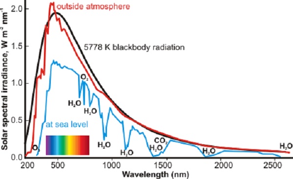
Part 11.10: Atmospheric Effects
Section Twelve: Aerosols
Part 12.1: Definitions
Part 12.2: Size Distribution
Part 12.3: Aerosol Motion in fluid
Part 12.4: Dynamics of Aerosols
Part 12.5: Aerosol Coagulation
Part 12.6: Atmospheric Aerosols
Section Thirteen: Statistical Physics and Thermodynamics
Part 13.1: Statistical Mechanics
Part 13.2: Maxwell-Boltzmann Distribution
Part 13.3: Brownian Motion
Section Fourteen: Geophysics of the Earth
Part 14.1: The Shape of the Earth
Part 14.1.1: The Geoid
Part 14.1.2: Relationship to GPS/GNSS
Part 14.2: Gravitational Field
Part 14.2.1: Introductory Remarks
Part 14.2.2: Classical Mechanical Theory
Part 14.3: Magnetic Field
Part 14.4: Electricity
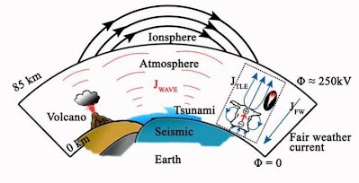
Part 14.4.1: Static Electrical Field
Part 14.4.2: Atmospheric Potential Gradient
Section Fifteen: The Atmosphere
Layers of the Earth's Atmosphere
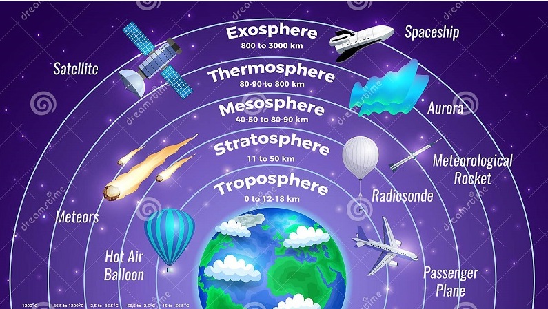
Part 15.1: The Troposphere
Part 15.2: The Stratosphere
Part 15.3: The Mesosphere
Part 15.4: The Thermosphere
Part 15.5: The Exosphere
Part 15.6: The Ionosphere
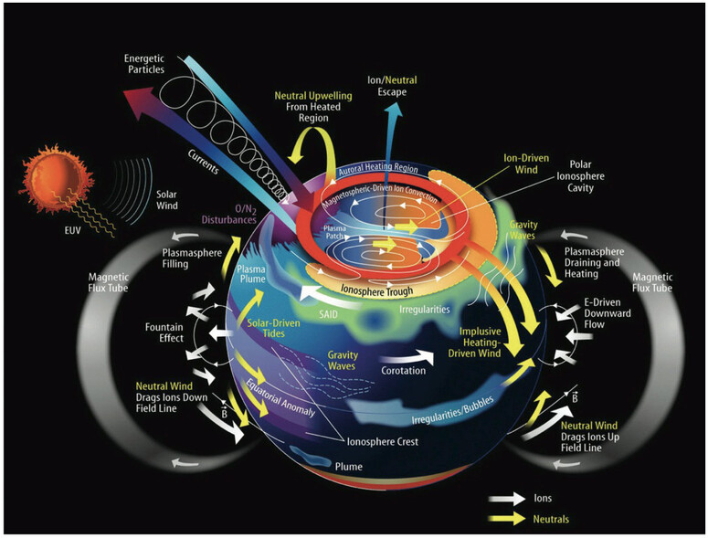
Part 15.7: The Ozone Layer
Part 15.8: The Homosphere
Part 15.9: The Hydrosphere
Part 15.10: Earth's Boundary Layer
Part 15.3: Atmospheric Thermodynamics
Section Sixteen: Turbulence
Part 16.1: Examples of Turbulence
Part 16.2: Characteristics of Turbulence
Turbulent flow is always rotational and three dimensional. For example, atmospheric cyclones are rotational but their substantially two-dimensional shapes do not allow vortex generation and so are turbulent. On the other hand, oceanic flows are dispersive but essentially non rotational and therefore are not turbulent. Part 16.3: Onset of Turbulence
While there is no theorem directly relating the non-dimensional Reynolds number to turbulence, flows at Reynolds numbers larger than 5000 are typically (but not necessarily) turbulent, while those at low Reynolds numbers usually remain laminar.
Part 16.4: Vorticity
A key concept in the dynamics of turbulent flow is the vorticity, a vector that describes the local rotary motion at a point in the fluid, as would be perceived by an observer that moves along with it. Conceptually, the vorticity could be observed by placing a tiny rough ball at the point in question, free to move with the fluid, and observing how it rotates about its center. The direction of the vorticity vector is defined to be the direction of the axis of rotation of this imaginary ball (according to the right-hand rule) while its length is twice the ball's angular velocity.
Mathematically, the vorticity is defined as the curl of the velocity field of the fluid, usually denoted by $ {\displaystyle {\vec {\omega }}} $ and expressed by the vector analysis formula $ {\displaystyle \nabla \times {\vec {\mathit {u}}}} $ , where $ {\displaystyle \nabla } $ is the nabla operator and $ {\displaystyle {\vec {\mathit {u}}}} $ .
The local rotation measured by the vorticity $ {\displaystyle {\vec {\omega }}} $ must not be confused with the angular velocity vector of that portion of the fluid with respect to the external environment or to any fixed axis. In a vortex, in particular, $ {\displaystyle {\vec {\omega }}} $ may be opposite to the mean angular velocity vector of the fluid relative to the vortex's axis.
In the absence of external forces, a vortex usually evolves fairly quickly toward the irrotational flow pattern, where the flow velocity $ {\displaystyle u} $ is inversely proportional to the distance $ {\displaystyle r} $ .
For an irrotational vortex, the circulation is zero along any closed contour that does not enclose the vortex axis; and has a fixed value, $ {\displaystyle \Gamma} $ , for any contour that does enclose the axis once. The tangential component of the particle velocity is then $ {\displaystyle u_{\theta }={\tfrac {\Gamma }{2\pi r}}} $ . The angular momentum per unit mass relative to the vortex axis is therefore constant, $ {\displaystyle ru_{\theta }={\tfrac {\Gamma }{2\pi }}} $ .
The ideal irrotational vortex flow in free space is not physically realizable, since it would imply that the particle speed (and hence the force needed to keep particles in their circular paths) would grow without bound as one approaches the vortex axis. Indeed, in real vortices there is always a core region surrounding the axis where the particle velocity stops increasing and then decreases to zero as $ {\displaystyle r} $ goes to zero. Within that region, the flow is no longer irrotational: the vorticity $ {\displaystyle {\vec {\omega }}} $ becomes non-zero, with direction roughly parallel to the vortex axis. The Rankine vortex is a model that assumes a rigid-body rotational flow where $ {\displaystyle r} $ is less than a fixed distance $ {\displaystyle r_ \theta} $ , and irrotational flow outside that core regions.
In a viscous fluid, irrotational flow contains viscous dissipation everywhere, yet there are no net viscous forces, only viscous stresses. Due to the dissipation, this means that sustaining an irrotational viscous vortex requires continuous input of work at the core (for example, by steadily turning a cylinder at the core). In free space there is no energy input at the core, and thus the compact vorticity held in the core will naturally diffuse outwards, converting the core to a gradually-slowing and gradually-growing rigid-body flow, surrounded by the original irrotational flow. Such a decaying irrotational vortex has an exact solution of the viscous Navier–Stokes equations, known as a Lamb–Oseen vortex.
A rotational vortex – a vortex that rotates in the same way as a rigid body – cannot exist indefinitely in that state except through the application of some extra force, that is not generated by the fluid motion itself. It has non-zero vorticity everywhere outside the core. Rotational vortices are also called rigid-body vortices or forced vortices.
Part 16.4.1: Vortex Formation
Vortex structures are defined by their vorticity, the local rotation rate of fluid particles. They can be formed via the phenomenon known as boundary layer separation which can occur when a fluid moves over a surface and experiences a rapid acceleration from the fluid velocity to zero due to the no-slip condition. This rapid negative acceleration creates a boundary layer which causes a local rotation of fluid at the wall (i.e. vorticity) which is referred to as the wall shear rate. The thickness of this boundary layer is proportional to $ {\displaystyle \surd (vt)} $ (where $ {\displaystyle v} $ is the free stream fluid velocity and $ {\displaystyle t} $ is time).
If the diameter or thickness of the vessel or fluid is less than the boundary layer thickness then the boundary layer will not separate and vortices will not form. However, when the boundary layer does grow beyond this critical boundary layer thickness then separation will occur which will generate vortices.
This boundary layer separation can also occur in the presence of combatting pressure gradients (i.e. a pressure that develops downstream). This is present in curved surfaces and general geometry changes like a convex surface. A unique example of severe geometric changes is at the trailing edge of a bluff body where the fluid flow deceleration, and therefore boundary layer and vortex formation, is located.
Part 16.4.2: Vortex Geometry
In a stationary vortex, the typical streamline (a line that is everywhere tangent to the flow velocity vector) is a closed loop surrounding the axis and each vortex line (a line that is everywhere tangent to the vorticity vector) is roughly parallel to the axis. A surface that is everywhere tangent to both flow velocity and vorticity is called a vortex tube. In general, vortex tubes are nested around the axis of rotation. The axis itself is one of the vortex lines, a limiting case of a vortex tube with zero diameter.
According to Helmholtz's theorems, a vortex line cannot start or end in the fluid – except momentarily, in non-steady flow, while the vortex is forming or dissipating. In general, vortex lines (in particular, the axis line) are either closed loops or end at the boundary of the fluid. A whirlpool is an example of the latter, namely a vortex in a body of water whose axis ends at the free surface. A vortex tube whose vortex lines are all closed will be a closed torus-like surface.
A newly created vortex will promptly extend and bend so as to eliminate any open-ended vortex lines. For example, when an airplane engine is started, a vortex usually forms ahead of each propeller, or the turbofan of each jet engine. One end of the vortex line is attached to the engine, while the other end usually stretches out and bends until it reaches the ground.
When vortices are made visible by smoke or ink trails, they may seem to have spiral pathlines or streamlines. However, this appearance is often an illusion and the fluid particles are moving in closed paths. The spiral streaks that are taken to be streamlines are in fact clouds of the marker fluid that originally spanned several vortex tubes and were stretched into spiral shapes by the non-uniform flow velocity distribution.
The fluid motion in a vortex creates a dynamic pressure (in addition to any hydrostatic pressure) that is lowest in the core region, closest to the axis, and increases as one moves away from it, in accordance with Bernoulli's principle. One can say that it is the gradient of this pressure that forces the fluid to follow a curved path around the axis.
In a rigid-body vortex flow of a fluid with constant density, the dynamic pressure is proportional to the square of the distance r from the axis. In a constant gravity field, the free surface of the liquid, if present, is a concave paraboloid.
The core of a vortex in air is sometimes visible because water vapor condenses as the low pressure of the core causes adiabatic cooling; the funnel of a tornado is an example. When a vortex line ends at a boundary surface, the reduced pressure may also draw matter from that surface into the core. For example, a dust devil is a column of dust picked up by the core of an air vortex attached to the ground. A vortex that ends at the free surface of a body of water (like the whirlpool that often forms over a bathtub drain) may draw a column of air down the core.
Vortices in the Earth's atmosphere are important phenomena for meteorology. They include mesocyclones on the scale of a few miles, tornadoes, waterspouts, and hurricanes. These vortices are often driven by temperature and humidity variations with altitude. The sense of rotation of hurricanes is influenced by the Earth's rotation. Another example is the Polar vortex, a persistent, large-scale cyclone centered near the Earth's poles, in the middle and upper troposphere and the stratosphere.
Section Seventeen: Dynamic Meteorology
Dynamic meteorology is the study of those motions of the atmosphere that are associated with the production of the circulation models, including the dynamics of air and moisture. For all such motions the discrete molecular nature of the atmosphere can be ignored, and the atmosphere can be regarded as a continuous fluid medium, or continuum. A “point” in the continuum is regarded as a volume element that is very small compared with the volume of atmosphere under consideration, but still contains a large number of molecules.
The expressions air parcel and air particle are both commonly used to refer to such a point. The various physical quantities that characterize the state of the atmosphere (e.g.,pressure, density, temperature) are assumed to have unique values at each point in the atmospheric continuum. Moreover, these field variables and their derivatives are assumed to be continuous functions of space and time. The fundamental laws of fluid mechanics and thermodynamics, which govern the motions of the atmosphere, may then be expressed in terms of partial differential equations involving the field variables as dependent variables and space and time as independent variables.
The general set of partial differential equations governing the motions of the atmosphere in the boundary layer with which we will be concerned is extremely complex. Because the planetary boundary layer is controlled by turbulent flow no general solutions are known to exist. To acquire an understanding of the physical role of atmospheric motions in determining the dynamics of the plume generated by the ionization of moleacules in the lower layer of the earth plaanetary layer, it is necessary to develop models based on systematic simplification of the fundamental governing equations. As shown in later sections, the development of models appropriate to the particular atmospheric motion systems requires careful consideration of the scales of motion involved.
Part 17.1: Atmospheric Forces
The motions of the atmosphere are governed by the fundamental physical laws of conservation of mass, momentum, and energy. These principles are applied to a small volume element of the atmosphere in order to obtain the governing equations. However, before deriving the complete momentum equation it is useful to discuss the nature of the forces that influence atmospheric motions.
These forces can be classified as either body forces or surface forces. Body forces act on the center of mass of a fluid parcel; they have magnitudes proportional to the mass of the parcel. Gravity is an example of a body force. Surface forces act across the boundary surface separating a fluid parcel from its surroundings. The surface forces involved in our model are the surface tension forces on a water droplet. The special character of the surface tension of water is an important consideration in the creation of precipitation.
The body forces which will form the basis of our discussion on the use of negative ions to generate water droplets are the forces generated by the static electrical potential which controls the planetary electrical circuits.
Newton’s second law of motion states that the rate of change of momentum (i.e., the acceleration) of an object, as measured relative to coordinates fixed in space, equals the sum of all the forces acting. For the development of our model, the forces that are of primary concern are the pressure gradient force, the gravitational force, and friction. These fundamental forces are the subject of the present section. If, as is the usual case, the motion is referred to a coordinate system rotating with the earth, Newton’s second law may still be applied provided that certain apparent forces, the centrifugal force and the Coriolis force, are included among the forces acting.
Part 17.2: Pressure Gradient Forces
In fluid mechanics, the pressure-gradient force is the force that results when there is a difference in pressure across a surface. In general, a pressure is a force per unit area, across a surface. A difference in pressure across a surface then implies a difference in force, which can result in an acceleration according to Newton's second law of motion.
The resulting force is always directed from the region of higher-pressure to the region of lower-pressure. When a fluid is in an equilibrium state (i.e. there are no net forces, and no acceleration), the system is referred to as being in hydrostatic equilibrium. In the case of atmospheres, the pressure-gradient force is balanced by the gravitational force, maintaining hydrostatic equilibrium. In Earth's atmosphere, for example, air pressure decreases at altitudes above Earth's surface, thus providing a pressure-gradient force which counteracts the force of gravity on the atmosphere.
Mathematical Formalism: Consider a small cubic parcel of fluid with a density $ {\displaystyle \rho } $ , a height $ {\displaystyle dz,} $ and a surface area $ {\displaystyle dA} $ . The mass of the parcel can be expressed as, $ {\displaystyle m=\rho \,dA\,dz} $ . Using Newton's second law, $ {\displaystyle F=ma} $ , we can then examine a pressure difference $ {\displaystyle dP} $ (assumed to be only in the $ {\displaystyle z} $ -direction) to find the resulting force, $ {\displaystyle F=-dP\,dA=\rho a\,dA\,dz} $ .
The acceleration resulting from the pressure gradient is then:
$$ {\displaystyle a=-{\frac {1}{\rho }}{\frac {dP}{dz}}.} $$The effects of the pressure gradient are usually expressed in terms of an acceleration instead of a force. We can express the acceleration more precisely, for a general pressure $ {\displaystyle P} $ as:
$$ {\displaystyle {\vec {a}}=-{\frac {1}{\rho }}{\vec {\nabla }}P.} $$The direction of the resulting force (acceleration) is thus in the opposite direction of the most rapid increase of pressure.
Part 17.2.1: Geostrophic Balance
A useful heuristic is to imagine air starting from rest, experiencing a force directed from areas of high pressure toward areas of low pressure, called the pressure gradient force. If the air began to move in response to that force, however, the Coriolis "force" would deflect it, to the right of the motion in the northern hemisphere or to the left in the southern hemisphere.
As the air accelerated, the deflection would increase until the Coriolis force's strength and direction balanced the pressure gradient force, a state called geostrophic balance. At this point, the flow is no longer moving from high to low pressure, but instead moves along isobars. Geostrophic balance helps to explain why, in the northern hemisphere, low-pressure systems (or cyclones) spin counterclockwise and high-pressure systems (or anticyclones) spin clockwise, and the opposite in the southern hemisphere.
Part 17.2.2: Geostrophic Current
Flow of ocean water is also largely geostrophic. Just as multiple weather balloons that measure pressure as a function of height in the atmosphere are used to map the atmospheric pressure field and infer the geostrophic wind, measurements of density as a function of depth in the ocean are used to infer geostrophic currents. Satellite altimeters are also used to measure sea surface height anomaly, which permits a calculation of the geostrophic current at the surface.
Part 17.3: Viscous Forces
Viscosity is the material property which relates the viscous stresses in a material to the rate of change of a deformation (the strain rate). Although it applies to general flows, it is easier to visualize and define in a simple shearing flow. Viscous forces dominate in the lower part of the planetary boundary layer where our equipment operates.
In many fluids, the flow velocity is observed to vary linearly from zero at the bottom to $ {\displaystyle u} $ at the top of the boundary layer. Moreover, the magnitude of the force, $ {\displaystyle F} $ , acting on the boundary layer, at the intersection with the flow stream is found to be proportional to the velocity of the fluid stream $ {\displaystyle u} $ and inversely proportional to their separation $ {\displaystyle y} $ :
$$ {\displaystyle F=\mu A{\frac {u}{y}}.} $$ .The proportionality factor is the dynamic viscosity of the fluid, often simply referred to as the viscosity. It is denoted by the Greek letter $ {\displaystyle mu (\mu)} $ . The dynamic viscosity has the dimensions $ {\displaystyle \mathrm {(mass/length)/time} } $ , therefore resulting in the SI units and the derived units:
$$ {\displaystyle [\mu ]={\frac {\rm {kg}}{\rm {m\cdot s}}}={\frac {\rm {N}}{\rm {m^{2}}}}\cdot s={\rm {Pa\cdot s}}= pressure \, multiplied \, by \, time.} $$The aforementioned ratio $ {\displaystyle u/y} $ is called the rate of shear deformation or shear velocity, and is the derivative of the fluid speed in the direction perpendicular to the normal vector of the surface of the earth. If the velocity does not vary linearly with $ {\displaystyle y} $ , then the appropriate generalization is:
$$ {\displaystyle \tau =\mu {\frac {\partial u}{\partial y}},} $$Where $ {\displaystyle \tau =F/A} $ , and $ {\displaystyle \partial u/\partial y} $ is the local shear velocity. This expression is referred to as Newton's law of viscosity. In shearing flows with planar symmetry, it is what defines $ {\displaystyle \mu } $ .
Use of the Greek letter ($ {\displaystyle \mu }) $ for the dynamic viscosity (sometimes also called the absolute viscosity) is common among engineers. However, the Greek letter ($ {\displaystyle \eta } $ ) is also used by chemists, physicists, and the IUPAC. The viscosity $ {\displaystyle \mu } $ is sometimes also called the shear viscosity.
The force of viscosity on a small sphere moving through a viscous fluid is given by: $$ {\displaystyle F_{\rm {d}}=6\pi \mu Rv} $$
Where:
$ {\displaystyle V(t)} $ is the particle speed at time t
$ {\displaystyle V_{f}} $ is the final particle speed
$ {\displaystyle V_{0}} $ is the initial particle speed
$ {\displaystyle F_{\rm {d}}} $ is the frictional force between the fluid and particle.
$ {\displaystyle \mu} $ is the dynamic viscosity
$ {\displaystyle R} $ is the radius of the spherical object
$ {\displaystyle v} $ is the flow velocity relative to the object.
Part 17.4: Gravitational Forces
The gravity of Earth, denoted by $ {\displaystyle g,} $ is the net acceleration that is imparted to objects due to the combined effect of gravitation (from mass distribution within Earth) and the centrifugal force (from the Earth's rotation). It is a vector quantity, whose direction coincides with a plumb bob and strength or magnitude is given by the norm $ {\displaystyle g=\|{\mathit {\mathbf {g} }}\|} $ .
Part 17.4.1: Conventional Values
In SI units this acceleration is expressed in metres per second squared. Near Earth's surface, the gravity acceleration is approximately $ {\displaystyle 9.81 m/s^2 } $ . The precise strength of Earth's gravity varies depending on location. The nominal "average" value at Earth's surface, known as standard gravity is, by definition, $ {\displaystyle 9.80665 m/s^2} $ .This definition is thus not a value of any particular place or carefully worked out average, but an agreement for a value to use if a better actual local value is not known or not important. It is also used to define the units kilogram force and pound force.
The weight of an object on Earth's surface is the downwards force on that object, given by Newton's second law. Gravitational acceleration contributes to the total gravity acceleration, but other factors, such as the rotation of Earth, also contribute, and, therefore, affect the weight of the object.
A non-rotating perfect sphere of uniform mass density, or whose density varies solely with distance from the centre (spherical symmetry), would produce a gravitational field of uniform magnitude at all points on its surface. The Earth is rotating but is not spherically symmetric; rather, it is an oblate spheroid. There are consequently slight deviations in the magnitude of gravity across its surface.
Part 17.4.2: Latitude
The Earth is rotating so it's surface is not an inertial frame of reference. At latitudes nearer the Equator, the outward centrifugal force produced by Earth's rotation is larger than at polar latitudes. This counteracts the Earth's gravity to a small degree – up to a maximum of 0.3% at the Equator – and reduces the apparent downward acceleration of falling objects.
The second major reason for the difference in gravity at different latitudes is that the Earth's equatorial bulge (itself also caused by centrifugal force from rotation) causes objects at the Equator to be farther from the planet's center than objects at the poles. Because the force due to gravitational attraction between two bodies varies inversely with the square of the distance between them, an object at the Equator experiences a weaker gravitational pull than an object on the pole.
In combination, the equatorial bulge and the effects of the surface centrifugal force due to rotation mean that sea-level gravity increases from about $ {\displaystyle 9.780 m/s^2 } $ the Equator to about $ {\displaystyle 9.832 m/s^2 } $ at the poles.
Part 17.4.3: Altitude
The following formula approximates the Earth's gravity variation with altitude:
$$ {\displaystyle g_{h}=g_{0}\left({\frac {R_{\mathrm {e} }}{R_{\mathrm {e} }+h}}\right)^{2}} $$Where:
$ {\displaystyle g_h} $ is the gravitational acceleration at height h above sea level
$ {\displaystyle R_e} $ is the Earth's mean radius.
$ {\displaystyle g_0} $ is the standard gravitational acceleration.
Part 17.5: Electrostatic Forces
The electrostatic force is the force of attraction or repulsion between charged particles. It is also called Coulomb’s force or Coulomb’s interaction. In the atmospheric physics domain the electrostatic force is the prime cause of the electric potential between the earth and the upper part of the troposphere.
Part 17.5.1: Electrostatic Approximation
The validity of the electrostatic approximation rests on the assumption that the electric field is irrotational:
$$ {\displaystyle {\vec {\nabla }}\times {\vec {E}}=0.} $$ .From Faraday's law, this assumption implies the absence or near-absence of time-varying magnetic fields:
$$ {\displaystyle {\partial {\vec {B}} \over \partial t}=0} $$In other words, electrostatics does not require the absence of magnetic fields or electric currents. Rather, if magnetic fields or electric currents do exist, they must not change with time, or in the worst-case, they must change with time only very slowly. In some problems, both electrostatics and magnetostatics may be required for accurate predictions, but the coupling between the two can still be ignored.
Part 17.5.2: Electrostatic Potential
When the electric field is irrotational, it is possible to express the electric field as the gradient of a scalar function, $ {\displaystyle \phi } $ , called the electrostatic potential (also known as the voltage). An electric field, $ {\displaystyle E} $ , points from regions of high electric potential to regions of low electric potential, expressed mathematically as:
$$ {\displaystyle {\vec {E}}=-{\vec {\nabla }}\phi } $$The gradient theorem can be used to establish that the electrostatic potential is the amount of work per unit charge required to move a charge from point $ {\displaystyle a} $ to point $ {\displaystyle b} $ with the following line integral:
$$ {\displaystyle -\int _{a}^{b}{{\vec {E}}\cdot \mathrm {d} {\vec {\ell }}}=\phi ({\vec {b}})-\phi ({\vec {a}}).} $$From these equations, we see that the electric potential is constant in any region for which the electric field vanishes.
Part 17.5.3: Electrostatic Energy
A test particle's potential energy, $ {\displaystyle U_{\mathrm {E} }^{\text{single}}} $ , can be calculated from a line integral of the work, $ {\displaystyle q_{n}{\vec {E}}\cdot \mathrm {d} {\vec {\ell }}} $ . We integrate from a point at infinity, and assume a collection of $ {\displaystyle N} $ particles of charge $ {\displaystyle Q_{n}} $ , are already situated at the points $ {\displaystyle {\vec {r}}_{i}} $ . This potential energy (in Joules) is:
$$ {\displaystyle U_{\mathrm {E} }^{\text{single}}=q\phi ({\vec {r}})={\frac {q}{4\pi \varepsilon _{0}}}\sum _{i=1}^{N}{\frac {Q_{i}}{\left\|{\mathcal {{\vec {R}}_{i}}}\right\|}}} $$Where: $ {\displaystyle {\vec {\mathcal {R_{i}}}}={\vec {r}}-{\vec {r}}_{i}} $ is the distance of each charge $ {\displaystyle Q_{i}} $ from the test charge $ {\displaystyle q} $ , which situated at the point $ {\displaystyle i} $ , and $ {\displaystyle \phi ({\vec {r}})} $ is the electric potential that would be at $ {\displaystyle {\vec {r}}} $ if the test charge were not present. If only two charges are present, the potential energy is $ {\displaystyle k_{\text{e}}Q_{1}Q_{2}/r} $ . The total electric potential energy due a collection of $ {\displaystyle N} $ charges is calculating by assembling these particles one at a time:
$$ {\displaystyle U_{\mathrm {E} }^{\text{total}}={\frac {1}{4\pi \varepsilon _{0}}}\sum _{j=1}^{N}Q_{j}\sum _{i=1}^{j-1}{\frac {Q_{i}}{r_{ij}}}={\frac {1}{2}}\sum _{i=1}^{N}Q_{i}\phi _{i},} $$Where the following sum from, $ {\displaystyle j = 1} $ to $ {\displaystyle N} $ , excludes $ {\displaystyle i = j} $ :
$$ {\displaystyle \phi_{i}={\frac {1}{4\pi \varepsilon _{0}}}\sum _{\stackrel {j=1}{j\neq i}}^{N}{\frac {Q_{j}}{r_{ij}}}.} $$This electric potential, $ {\displaystyle \phi _{i}} $ is what would be measured at $ {\displaystyle {\vec {r}}_{i}} $ if the charge $ {\displaystyle Q_{i}} $ were missing. This formula obviously excludes the (infinite) energy that would be required to assemble each point charge from a disperse cloud of charge. The sum over charges can be converted into an integral over charge density using the prescription $ {\textstyle \sum (\cdots )\rightarrow \int (\cdots )\rho \,\mathrm {d} ^{3}r} $
$$ {\displaystyle U_{\mathrm {E} }^{\text{total}}={\frac {1}{2}}\int \rho ({\vec {r}})\phi ({\vec {r}})\,\mathrm {d} ^{3}r={\frac {\varepsilon _{0}}{2}}\int \left|{\mathbf {E} }\right|^{2}\,\mathrm {d} ^{3}r,} $$This second expression for electrostatic energy uses the fact that the electric field is the negative gradient of the electric potential, as well as the vector calculus identities in a way that resembles integration by parts. These two integrals for electric field energy seem to indicate two mutually exclusive formulas for electrostatic energy density, namely $ {\textstyle {\frac {1}{2}} \rho \phi } $ and $ {\textstyle {\frac {1}{2}}\varepsilon _{0}E^{2}} $ ; they yield equal values for the total electrostatic energy only if both are integrated over all space.
Part 17.5.4: Electrostatic Pressure
On a conductor, a surface charge will experience a force in the presence of an electric field. This force is the average of the discontinuous electric field at the surface charge. This average in terms of the field just outside the surface amounts to:
$$ {\displaystyle P={\frac {\varepsilon _{0}}{2}}E^{2},} $$This pressure tends to draw the conductor into the field, regardless of the sign of the surface charge.
Part 17.6: Magnetostatic Force
Magnetostatics is the study of magnetic fields in systems where the currents are steady. The magnetization need not be static. Magnetostatics is even a good approximation when the currents are not static – as long as the currents do not alternate rapidly.
Current Sources If all currents in a system are known (i.e., if a complete description of the current density $ {\displaystyle \mathbf {J} (\mathbf {r} )} $ is available) then the magnetic field can be determined, at a positionr, from the currents by the Biot–Savart equation:
$$ {\displaystyle \mathbf {B} (\mathbf {r} )={\frac {\mu _{0}}{4\pi }}\int {{\frac {\mathbf {J} (\mathbf {r} ')\times \left(\mathbf {r} -\mathbf {r} '\right)}{|\mathbf {r} -\mathbf {r} '|^{3}}}\mathrm {d} ^{3}\mathbf {r} '}} $$This technique works well for problems where the medium is a vacuum or air or some similar material with a relative permeability of 1. This includes the atmosphere surrounding the earth. Since this equation is primarily used to solve linear problems, the contributions can be added. For a very difficult geometry, numerical integration may be used.
The value of $ {\displaystyle \mathbf {B} } $ can be found from the magnetic potential. Since the divergence of the magnetic flux density is always zero:
$$ {\displaystyle \mathbf {B} =\nabla \times \mathbf {A} } $$And the relation of the vector potential to current is:
$$ {\displaystyle \mathbf {A} (\mathbf {r} )={\frac {\mu _{0}}{4\pi }}\int {{\frac {\mathbf {J(\mathbf {r} ')} }{|\mathbf {r} -\mathbf {r} '|}}\mathrm {d} ^{3}\mathbf {r} '}.} $$Magnetization: Strongly magnetic materials have a magnetization that is primarily due to electron spin. In such materials the magnetization must be explicitly included using the relation:
$$ {\displaystyle \mathbf {B} =\mu _{0}(\mathbf {M} +\mathbf {H} ).} $$Except in the case of conductors, electric currents can be ignored. Then Ampère's law is simply:
$$ {\displaystyle \nabla \times \mathbf {H} =0.} $$This has the general solution:
$$ {\displaystyle \mathbf {H} =-\nabla \Phi _{M},} $$Where $ {\displaystyle \Phi _{M}} $ is a scalar potential.
Substituting this in Gauss's law gives:
$$ {\displaystyle \nabla ^{2}\Phi _{M}=\nabla \cdot \mathbf {M} .} $$Thus, the divergence of the magnetization, $ {\displaystyle \nabla \cdot \mathbf {M} ,} $ has a role analogous to the electric charge in electrostatics.
The vector potential method can also be employed with an effective current density:
$$ {\displaystyle \mathbf {J_{M}} =\nabla \times \mathbf {M} .} $$Part 17.7: Rotational Dynamics
In order to study the dynamics of the earth one must first have an understanding of the laws governing the motion of rigid bodies. Rrigid-body dynamics studies the movement of systems of interconnected bodies under the action of external forces. The assumption that the bodies are rigid (i.e. they do not deform under the action of applied forces) simplifies analysis, by reducing the parameters that describe the configuration of the system to the translation and rotation of reference frames attached to each body.
The dynamics of a rigid body system is described by the application of Newton's second law or in their derivative form, Lagrangian mechanics. The solution of these equations of motion provides a description of the position, the motion and the acceleration of the individual components of the system, and overall the system itself (in our case the rotation of the earth), as a function of time. The formulation and solution of planetary circulation system depend on an understanding of rigid body dynamics.
Part 17.7.1: Newton's Second Law in Three Dimensions
To consider rigid body dynamics in three-dimensional space, Newton's second law must be extended to define the relationship between the movement of a rigid body and the system of forces and torques that act on it.
Newton formulated his second law for a particle as, "The change of motion of an object is proportional to the force impressed and is made in the direction of the straight line in which the force is impressed." Because Newton generally referred to mass times velocity as the "motion" of a particle, the phrase "change of motion" refers to the mass times acceleration of the particle, and so this law is usually written as:
$$ {\displaystyle \mathbf {F} =m\mathbf {a}} $$Where $ {\displaystyle \mathbf {F}} $ is understood to be the only external force acting on the particle, $ {\displaystyle m} $ is the mass of the particle, and $ {\displaystyle \mathbf {a}} $ is its acceleration vector. The extension of Newton's second law to rigid bodies is achieved by considering a rigid system of particles.
Part 17.7.2: Rigid System of Particles
If a system of $ {\displaystyle N} $ particles, $ {\displaystyle P_i} $ , $ {\displaystyle i = 1,...,N} $ , are assembled into a rigid body, then Newton's second law can be applied to each of the particles in the body.
If $ {\displaystyle \mathbf {F}_i} $ is the external force applied to particle $ {\displaystyle P_i} $ with mass $ {\displaystyle m_i} $ , then:
$$ {\displaystyle \mathbf {F} _{i}+\sum _{j=1}^{N}\mathbf {F} _{ij}=m_{i}\mathbf {a} _{i},\quad i=1,\ldots ,N,} $$Where $ {\displaystyle \mathbf {F}_{ij}} $ is the internal force of particle $ {\displaystyle P_j} $ acting on particle $ {\displaystyle P_i} $ that maintains the constant distance between these particles.
An important simplification to these force equations is obtained by introducing the resultant force and torque that acts on the rigid system. This resultant force and torque is obtained by choosing one of the particles in the system as a reference point, $ {\displaystyle \mathbf {R},} $ where each of the external forces are applied with the addition of an associated torque. The resultant force $ {\displaystyle \mathbf {F}} $ and torque $ {\displaystyle \mathbf {T}} $ are given by the formulas:
$$ {\displaystyle \mathbf {F} =\sum _{i=1}^{N}\mathbf {F} _{i},\quad \mathbf {T} =\sum _{i=1}^{N}(\mathbf {R} _{i}-\mathbf {R} )\times \mathbf {F} _{i},} $$Where $ {\displaystyle \mathbf {R}_i} $ is the vector that defines the position of particle $ {\displaystyle \mathbf {P}_i} $ .
Newton's second law for a particle combines with these formulas for the resultant force and torque to yield:
$$ {\displaystyle \mathbf {F} =\sum _{i=1}^{N}m_{i}\mathbf {a} _{i},\quad \mathbf {T} =\sum _{i=1}^{N}(\mathbf {R} _{i}-\mathbf {R} )\times (m_{i}\mathbf {a} _{i}),} $$Where the internal forces $ {\displaystyle \mathbf {F}_{ij}} $ cancel in pairs. The kinematics of a rigid body yields the formula for the acceleration of the particle $ {\displaystyle \mathbf {P}_i} $ in terms of the position $ {\displaystyle \mathbf {R} } $ and acceleration $ {\displaystyle \mathbf {a}} $ of the reference particle as well as the angular velocity vector $ {\displaystyle \omega } $ and angular acceleration vector $ {\displaystyle \alpha } $ α of the rigid system of particles as:
$$ {\displaystyle \mathbf {a} _{i}=\alpha \times (\mathbf {R} _{i}-\mathbf {R} )+\omega \times (\omega \times (\mathbf {R} _{i}-\mathbf {R} ))+\mathbf {a} .} $$Part 17.7.3: Mass Properties
The mass properties of the rigid body are represented by its center of mass and inertia matrix. Choose the reference point $ {\displaystyle \mathbf {R} } $ so that it satisfies the condition:
$$ {\displaystyle \sum _{i=1}^{N}m_{i}(\mathbf {R} _{i}-\mathbf {R} )=0,} $$Then this point is known as the center of mass of the system.
The inertia matrix $ {\displaystyle [IR] } $ of the system relative to the reference point $ {\displaystyle \mathbf {R} } $ is defined by:
$$ {\displaystyle [I_{R}]=\sum _{i=1}^{N}m_{i}\left(\mathbf {I} \left(\mathbf {S} _{i}^{\textsf {T}}\mathbf {S} _{i}\right)-\mathbf {S} _{i}\mathbf {S} _{i}^{\textsf {T}}\right),} $$Where $ {\displaystyle \mathbf {S} _{i}} $ is the column vector $ {\displaystyle \mathbf {S} _{i}^{\textsf {T}}} $ is its transpose, and $ {\displaystyle \mathbf {I} } $ is the 3 by 3 identity matrix. $ {\displaystyle \mathbf {S} _{i}^{\textsf {T}}\mathbf {S} _{i}} $ is the scalar product of $ {\displaystyle \mathbf {S} _{i}} $ with itself, while $ {\displaystyle \mathbf {S} _{i}\mathbf {S} _{i}^{\textsf {T}}} $ is the tensor product of $ {\displaystyle \mathbf {S} _{i}} $ .
Part 17.5.4: Force-Torque Equations
Using the center of mass and inertia matrix, the force and torque equations for a single rigid body take the form:
$$ {\displaystyle \mathbf {F} =m\mathbf {a} ,\quad \mathbf {T} =[I_{R}]\alpha +\omega \times [I_{R}]\omega ,} $$And are known as Newton's second law of motion for a rigid body.
The dynamics of an interconnected system of rigid bodies, $ {\displaystyle {B_i, j = 1, ..., M,}} $ is formulated by isolating each rigid body and introducing the interaction forces. The resultant of the external and interaction forces on each body, yields the force-torque equations: $$ {\displaystyle \mathbf {F} _{j}=m_{j}\mathbf {a} _{j},\quad \mathbf {T} _{j}=[I_{R}]_{j}\alpha _{j}+\omega _{j}\times [I_{R}]_{j}\omega _{j},\quad j=1,\ldots ,M.} $$
Newton's formulation yields $ {\displaystyle 6M } $ equations that define the dynamics of a system of $ {\displaystyle M} $ rigid bodies.
Part 17.7.5: Rotation in Three Dimensions
A rotating object, whether under the influence of torques or not, may exhibit the behaviours of precession and nutation. The fundamental equation describing the behavior of a rotating solid body is Euler's equation of motion:
$$ {\displaystyle {\boldsymbol {\tau }}={\frac {D\mathbf {L} }{Dt}}={\frac {d\mathbf {L} }{dt}}+{\boldsymbol {\omega }}\times \mathbf {L} ={\frac {d(I{\boldsymbol {\omega }})}{dt}}+{\boldsymbol {\omega }}\times {I{\boldsymbol {\omega }}}=I{\boldsymbol {\alpha }}+{\boldsymbol {\omega }}\times {I{\boldsymbol {\omega }}}} $$Where the pseudovectors $ {\displaystyle {\boldsymbol {\tau }}} $ and $ {\displaystyle {\boldsymbol L}} $ are, respectively, the torques on the body and its angular momentum, the scalar $ {\displaystyle I} $ is its moment of inertia, the vector $ {\displaystyle {\boldsymbol {\Omega }}} $ is its angular velocity, the vector $ {\displaystyle {\boldsymbol {\alpha }}} $ is its angular acceleration, $ {\displaystyle D} $ is the differential in an inertial reference frame and $ {\displaystyle d} $ is the differential in a relative reference frame fixed with the body.
It follows from Euler's equation that a torque $ {\displaystyle {\boldsymbol {\tau }}} $ applied perpendicular to the axis of rotation, and therefore perpendicular to $ {\displaystyle {\boldsymbol {L}}} $ , results in a rotation about an axis perpendicular to both $ {\displaystyle {\boldsymbol {\tau }}} $ and $ {\displaystyle {\boldsymbol {L }}} $ . This motion is called precession. The angular velocity of precession $ {\displaystyle {\boldsymbol {\Omega}_P }} $ is given by the cross product:
$$ {\displaystyle {\boldsymbol {\tau }}={\boldsymbol {\Omega }}_{\mathrm {P} }\times \mathbf {L} .} $$Precession can be demonstrated by placing a spinning top with its axis horizontal and supported loosely (frictionless toward precession) at one end. Instead of falling, as might be expected, the top appears to defy gravity by remaining with its axis horizontal, when the other end of the axis is left unsupported and the free end of the axis slowly describes a circle in a horizontal plane, the resulting precession turning. This effect is explained by the above equations. The torque on the top is supplied by a couple of forces: gravity acting downward on the device's centre of mass, and an equal force acting upward to support one end of the device.
The rotation resulting from this torque is not downward, as might be intuitively expected, causing the device to fall, but perpendicular to both the gravitational torque (horizontal and perpendicular to the axis of rotation) and the axis of rotation (horizontal and outwards from the point of support), i.e., about a vertical axis, causing the device to rotate slowly about the supporting point.
Under a constant torque of magnitude $ {\displaystyle {\tau }} $ , the speed of precession $ {\displaystyle \Omega_p } $ is inversely proportional to $ {\displaystyle L} $ , the magnitude of its angular momentum:
$$ {\displaystyle \tau ={\mathit {\Omega }}_{\mathrm {P} }L\sin \theta ,} $$Where $ {\displaystyle \Theta } $ is the angle between the vectors $ {\displaystyle {\boldsymbol {\Omega}_P}} $ and $ {\displaystyle L} $ . Thus, if the top's spin slows down (for example, due to friction), its angular momentum decreases and so the rate of precession increases. This continues until the device is unable to rotate fast enough to support its own weight, when it stops precessing and falls off its support, mostly because friction against precession cause another precession that goes to cause the fall.
By convention, these three vectors - torque, spin, and precession - are all oriented with respect to each other according to the right-hand rule.
Part 17.8: Non-Inertial Forces
Part 17.8.1: Centrifugal Force
Centrifugal force is an outward force apparent in a rotating reference frame. It does not exist when a system is described relative to an inertial frame of reference.
All measurements of position and velocity must be made relative to some frame of reference. A reference frame that is at rest (or one that moves with no rotation and at constant velocity) relative to the "fixed stars" is generally taken to be an inertial frame. Any system can be analyzed in an inertial frame (and so with no centrifugal force). However, it is often more convenient to describe a rotating system by using a rotating frame—the calculations are simpler, and descriptions more intuitive. When this choice is made, fictitious forces, including the centrifugal force, arise.
Part 17.8.2: Reference Frame
In a reference frame rotating about an axis through its origin, all objects, regardless of their state of motion, appear to be under the influence of a radially (from the axis of rotation) outward force that is proportional to their mass, to the distance from the axis of rotation of the frame, and to the square of the angular velocity of the frame. This is the centrifugal force. As humans usually experience centrifugal force from within the rotating reference frame, e.g. on a merry-go-round or vehicle, this is much more well-known than centripetal force.
Motion relative to a rotating frame results in another fictitious force: the Coriolis force. If the rate of rotation of the frame changes, a third fictitious force (the Euler force) is required. These fictitious forces are necessary for the formulation of correct equations of motion in a rotating reference frame and allow Newton's laws to be used in their normal form in such a frame (with one exception: the fictitious forces do not obey Newton's third law: they have no equal and opposite counterparts). Newton's third law requires the counterparts to exist within the same frame of reference, hence centrifugal and centripetal force, which do not, are not action and reaction (as is sometimes erroneously contended).
The Earth constitutes a rotating reference frame because it rotates once every 23 hours and 56 minutes around its axis. Because the rotation is slow, the fictitious forces it produces are often small, and in everyday situations can generally be neglected. Even in calculations requiring high precision, the centrifugal force is generally not explicitly included, but rather lumped in with the gravitational force: the strength and direction of the local "gravity" at any point on the Earth's surface is actually a combination of gravitational and centrifugal forces. However, the fictitious forces can be of arbitrary size. For example, in an Earth-bound reference system, the fictitious force (the net of Coriolis and centrifugal forces) is enormous and is responsible for the Sun orbiting around the Earth (in the Earth-bound reference system). This is due to the large mass and velocity of the Sun (relative to the Earth).
Part 17.8.3: Weight of Objects
If an object is weighed with a simple spring balance at one of the Earth's poles, there are two forces acting on the object: the Earth's gravity, which acts in a downward direction, and the equal and opposite restoring force in the spring, acting upward. Since the object is stationary and not accelerating, there is no net force acting on the object and the force from the spring is equal in magnitude to the force of gravity on the object. In this case, the balance shows the value of the force of gravity on the object.
When the same object is weighed on the equator, the same two real forces act upon the object. However, the object is moving in a circular path as the Earth rotates and therefore experiencing a centripetal acceleration. When considered in an inertial frame (that is to say, one that is not rotating with the Earth), the non-zero acceleration means that force of gravity will not balance with the force from the spring. In order to have a net centripetal force, the magnitude of the restoring force of the spring must be less than the magnitude of force of gravity. Less restoring force in the spring is reflected on the scale as less weight — about 0.3% less at the equator than at the poles. In the Earth reference frame (in which the object being weighed is at rest), the object does not appear to be accelerating, however the two real forces, gravity and the force from the spring, are the same magnitude and do not balance. The centrifugal force must be included to make the sum of the forces be zero to match the apparent lack of acceleration.
Part 17.8.4: Time Derivative in Rotating Frame
In a rotating frame of reference, the time derivatives of any vector function $ {\displaystyle {\boldsymbol P}} $ of time—such as the velocity and acceleration vectors of an object—will differ from its time derivatives in the stationary frame. If $ {\displaystyle {\boldsymbol{ P_1, P_2, P_3}}}$ are the components of $ {\displaystyle {\boldsymbol P}} $ with respect to unit vectors $ {\displaystyle {\boldsymbol i, j,k}} $ directed along the axes of the rotating frame (i.e. $ {\displaystyle {\boldsymbol {P= P_1 i + P_2 j +P_3 k}}} $ ), then the first time derivative $ {\displaystyle [d{\boldsymbol P}/dt]} $ of $ {\displaystyle {\boldsymbol P}} $ with respect to the rotating frame is:
$$ {\displaystyle (d{\boldsymbol P_1}/dt) \boldsymbol i + (d \boldsymbol P_2/dt) \boldsymbol j + (d \boldsymbol P_3/dt) \boldsymbol k} $$ .If the absolute angular velocity of the rotating frame is $ {\displaystyle \omega} $ then the derivative $ {\displaystyle d{\boldsymbol P} /dt} $ of $ {\displaystyle {\boldsymbol P}} $ with respect to the stationary frame is related to $ {\displaystyle { [d{\boldsymbol P}/dt]}} $ by the equation:
$$ {\displaystyle {\frac {\operatorname {d} {\boldsymbol {P}}}{\operatorname {d} t}}=\left[{\frac {\operatorname {d} {\boldsymbol {P}}}{\operatorname {d} t}}\right]+{\boldsymbol {\omega }}\times {\boldsymbol {P}}\ ,}$$Where $ {\displaystyle \times }$ denotes the vector cross product. In other words, the rate of change of $ {\displaystyle {\boldsymbol P}} $ in the stationary frame is the sum of its apparent rate of change in the rotating frame and a rate of rotation $ {\displaystyle {\boldsymbol {\omega }}\times {\boldsymbol {P}}} $ attributable to the motion of the rotating frame. The vector $ {\displaystyle \boldsymbol \omega} $ has magnitude $ {\displaystyle \omega} $ equal to the rate of rotation and is directed along the axis of rotation according to the right-hand rule.
Part 17.8.5: Acceleration
Newton's law of motion for a particle of mass m written in vector form is:
$$ {\displaystyle {\boldsymbol {F}}=m{\boldsymbol {a}}\ ,} $$Where $ {\displaystyle {\boldsymbol {F}}} $ is the vector sum of the physical forces applied to the particle and $ {\displaystyle {\boldsymbol {a}}} $ is the absolute acceleration (that is, acceleration in an inertial frame) of the particle, given by:
$$ {\displaystyle {\boldsymbol {a}}={\frac {\operatorname {d} ^{2}{\boldsymbol {r}}}{\operatorname {d} t^{2}}}\ ,} $$Where $ {\displaystyle {\boldsymbol {r}}} $ is the position vector of the particle.
By applying the transformation above from the stationary to the rotating frame three times (twice to $ {\displaystyle {\frac {\operatorname {d} {\boldsymbol {r}}}{\operatorname {d} t}}}$ and once to $ {\displaystyle {\frac {\operatorname {d} }{\operatorname {d} t}}\left[{\frac {\operatorname {d} {\boldsymbol {r}}}{\operatorname {d} t}}\right]} $ ), the absolute acceleration of the particle can be written as:
$$ {\displaystyle {\begin{aligned}{\boldsymbol {a}}&={\frac {\operatorname {d} ^{2}{\boldsymbol {r}}}{\operatorname {d} t^{2}}}={\frac {\operatorname {d} }{\operatorname {d} t}}{\frac {\operatorname {d} {\boldsymbol {r}}}{\operatorname {d} t}}={\frac {\operatorname {d} }{\operatorname {d} t}}\left(\left[{\frac {\operatorname {d} {\boldsymbol {r}}}{\operatorname {d} t}}\right]+{\boldsymbol {\omega }}\times {\boldsymbol {r}}\ \right)\\&=\left[{\frac {\operatorname {d} ^{2}{\boldsymbol {r}}}{\operatorname {d} t^{2}}}\right]+{\boldsymbol {\omega }}\times \left[{\frac {\operatorname {d} {\boldsymbol {r}}}{\operatorname {d} t}}\right]+{\frac {\operatorname {d} {\boldsymbol {\omega }}}{\operatorname {d} t}}\times {\boldsymbol {r}}+{\boldsymbol {\omega }}\times {\frac {\operatorname {d} {\boldsymbol {r}}}{\operatorname {d} t}}\\&=\left[{\frac {\operatorname {d} ^{2}{\boldsymbol {r}}}{\operatorname {d} t^{2}}}\right]+{\boldsymbol {\omega }}\times \left[{\frac {\operatorname {d} {\boldsymbol {r}}}{\operatorname {d} t}}\right]+{\frac {\operatorname {d} {\boldsymbol {\omega }}}{\operatorname {d} t}}\times {\boldsymbol {r}}+{\boldsymbol {\omega }}\times \left(\left[{\frac {\operatorname {d} {\boldsymbol {r}}}{\operatorname {d} t}}\right]+{\boldsymbol {\omega }}\times {\boldsymbol {r}}\ \right)\\&=\left[{\frac {\operatorname {d} ^{2}{\boldsymbol {r}}}{\operatorname {d} t^{2}}}\right]+{\frac {\operatorname {d} {\boldsymbol {\omega }}}{\operatorname {d} t}}\times {\boldsymbol {r}}+2{\boldsymbol {\omega }}\times \left[{\frac {\operatorname {d} {\boldsymbol {r}}}{\operatorname {d} t}}\right]+{\boldsymbol {\omega }}\times ({\boldsymbol {\omega }}\times {\boldsymbol {r}})\ .\end{aligned}}} $$Part 17.8.6: Force
The apparent acceleration in the rotating frame is $ {\displaystyle \left[{\frac {d^{2}{\boldsymbol {r}}}{dt^{2}}}\right]} $. An observer unaware of the rotation would expect this to be zero in the absence of outside forces. However, Newton's laws of motion apply only in the inertial frame and describe dynamics in terms of the absolute acceleration $ {\displaystyle {\frac {d^{2}{\boldsymbol {r}}}{dt^{2}}}} $ . Therefore, the observer perceives the extra terms as contributions due to fictitious forces. These terms in the apparent acceleration are independent of mass; so it appears that each of these fictitious forces, like gravity, pulls on an object in proportion to its mass. When these forces are added, the equation of motion has the form:
$$ {\displaystyle {\boldsymbol {F}}-m{\frac {\operatorname {d} {\boldsymbol {\omega }}}{\operatorname {d} t}}\times {\boldsymbol {r}}-2m{\boldsymbol {\omega }}\times \left[{\frac {\operatorname {d} {\boldsymbol {r}}}{\operatorname {d} t}}\right]-m{\boldsymbol {\omega }}\times ({\boldsymbol {\omega }}\times {\boldsymbol {r}}) =m\left[{\frac {\operatorname {d} ^{2}{\boldsymbol {r}}}{\operatorname {d} t^{2}}}\right]\ .}$$From the perspective of the rotating frame, the additional force terms are experienced just like the real external forces and contribute to the apparent acceleration. The additional terms on the force side of the equation can be recognized as, reading from left to right, the Euler force $ {\displaystyle -m\operatorname {d} {\boldsymbol {\omega }}/\operatorname {d} t\times {\boldsymbol {r}}} $ , the Coriolis force $ {\displaystyle -2m{\boldsymbol {\omega }}\times \left[\operatorname {d} {\boldsymbol {r}}/\operatorname {d} t\right]} $ , and the centrifugal force $ {\displaystyle -m{\boldsymbol {\omega }}\times ({\boldsymbol {\omega }}\times {\boldsymbol {r}})} $ , respectively.
Unlike the other two fictitious forces, the centrifugal force always points radially outward from the axis of rotation of the rotating frame, with magnitude $ {\displaystyle m {{\omega}^2} r} $ , and unlike the Coriolis force in particular, it is independent of the motion of the particle in the rotating frame.
As expected, for a non-rotating inertial frame of reference $ {\displaystyle ({\boldsymbol {\omega }}=0)} $ the centrifugal force and all other fictitious forces disappear. Similarly, as the centrifugal force is proportional to the distance from object to the axis of rotation of the frame, the centrifugal force vanishes for objects that lie upon the axis.
Part 17.9: Centripetal Force
A centripetal force is a force that makes a body follow a curved path. Its direction is always orthogonal to the motion of the body and towards the fixed point of the instantaneous center of curvature of the path. Isaac Newton described it as "a force by which bodies are drawn or impelled, or in any way tend, towards a point as to a centre". In Newtonian mechanics, gravity provides the centripetal force causing astronomical orbits.
The magnitude of the centripetal force on an object of mass $ {\displaystyle m} $ moving at tangential speed $ {\displaystyle v} $ along a path with radius of curvature $ {\displaystyle r} $ is:
$$ {\displaystyle F_{c}=ma_{c}={\frac {mv^{2}}{r}}} $$ $$ {\displaystyle a_{c}=\lim _{\Delta t\to 0}{\frac {|\Delta {\textbf {v}}|}{\Delta t}}} $$Where $ {\displaystyle a_{c}}$ is the centripetal acceleration and $ {\displaystyle \Delta {\textbf {v}}} $ is the difference between the velocity vectors. Since the velocity vectors in the above diagram have constant magnitude and since each one is perpendicular to its respective position vector, simple vector subtraction implies two similar isosceles triangles with congruent angles – one comprising a base of $ {\displaystyle \Delta {\textbf {v}}} $ and a leg length of $ {\displaystyle v} $ , and the other a base of $ {\displaystyle \Delta {\textbf {r}}} $ (position vector difference) and a leg length of $ {\displaystyle r} $
$$ {\displaystyle {\frac {|\Delta {\textbf {v}}|}{v}}={\frac {|\Delta {\textbf {r}}|}{r}}} $$ $$ {\displaystyle |\Delta {\textbf {v}}|={\frac {v}{r}}|\Delta {\textbf {r}}|} $$Therefore, $ {\displaystyle |\Delta {\textbf {v}}|} $ can be substituted with $ {\displaystyle {\frac {v}{r}}|\Delta {\textbf {r}}|} $ :
$$ {\displaystyle a_{c}=\lim _{\Delta t\to 0}{\frac {|\Delta {\textbf {v}}|}{\Delta t}}={\frac {v}{r}}\lim _{\Delta t\to 0}{\frac {|\Delta {\textbf {r}}|}{\Delta t}}=\omega \lim _{\Delta t\to 0}{\frac {|\Delta {\textbf {r}}|}{\Delta t}}=v\omega ={\frac {v^{2}}{r}}} $$The direction of the force is toward the center of the circle in which the object is moving, or the osculating circle (the circle that best fits the local path of the object, if the path is not circular). The speed in the formula is squared, so twice the speed needs four times the force. The inverse relationship with the radius of curvature shows that half the radial distance requires twice the force. This force is also sometimes written in terms of the angular velocity ω of the object about the center of the circle, related to the tangential velocity by the formula:
$$ {\displaystyle v=\omega r} $$So that:
$$ {\displaystyle F_{c}=mr\omega ^{2}\,.} $$Expressed using the orbital period T for one revolution of the circle,
$$ {\displaystyle \omega ={\frac {2\pi }{T}}} $$The equation becomes:
$$ {\displaystyle F_{c}=mr\left({\frac {2\pi }{T}}\right)^{2}} $$Part 17.10: Coriolis Force
The Coriolis force is an inertial force that acts on objects in motion within a frame of reference that rotates with respect to an inertial frame. In a reference frame with clockwise rotation, the force acts to the left of the motion of the object. In one with counterclockwise rotation, the force acts to the right. Deflection of an object due to the Coriolis force is called the Coriolis effect.
Though recognized previously by others, the mathematical expression for the Coriolis force appeared in an 1835 paper by French scientist Gaspard-Gustave de Coriolis, in connection with the theory of water wheels. Early in the 20th century, the term Coriolis force began to be used in connection with atmospheric physics.
Newton's laws of motion describe the motion of an object in an inertial (non-accelerating) frame of reference. When Newton's laws are transformed to a rotating frame of reference, the Coriolis and centrifugal accelerations appear. When applied to objects with masses, the respective forces are proportional to their masses.
The magnitude of the Coriolis force is proportional to the rotation rate, and the magnitude of the centrifugal force is proportional to the square of the rotation rate.
The Coriolis force acts in a direction perpendicular to two quantities: the angular velocity of the rotating frame relative to the inertial frame and the velocity of the body relative to the rotating frame, and its magnitude is proportional to the object's speed in the rotating frame (more precisely, to the component of its velocity that is perpendicular to the axis of rotation).
The centrifugal force acts outwards in the radial direction and is proportional to the distance of the body from the axis of the rotating frame. These additional forces are termed inertial forces.
By introducing these forces to the rotating frame of reference, Newton's laws of motion can be applied to the rotating system as though it were an inertial system; these forces are correction factors that are not required in a non-rotating system.
In Newtonian mechanics, the equation of motion for an object in an inertial reference frame is:
$$ {\displaystyle {\boldsymbol {F}}=m{\boldsymbol {a}}} $$Where $ {\displaystyle {\boldsymbol {F}}} $ is the vector sum of the physical forces acting on the object, $ {\displaystyle m} $ is the mass of the object, and $ {\displaystyle {\boldsymbol {a}}} $ is the acceleration of the object relative to the inertial reference frame.
Transforming this equation to a reference frame rotating about a fixed axis through the origin with angular velocity $ {\displaystyle {\boldsymbol {\omega }}} $ having variable rotation rate, the equation takes the form:
$$ {\displaystyle {\boldsymbol {F}}-m{\frac {\operatorname {d} {\boldsymbol {\omega }}}{\operatorname {d} t}}\times {\boldsymbol {r'}}-2m{\boldsymbol {\omega }}\times {\boldsymbol {v'}}-m{\boldsymbol {\omega }}\times ({\boldsymbol {\omega }}\times {\boldsymbol {r'}}) =m {\boldsymbol {a'}}} $$Where:
$ {\displaystyle {\boldsymbol {F}}} $ is the vector sum of the physical forces acting on the object
$ {\displaystyle {\boldsymbol {\omega }}}$ is the angular velocity, of the rotating frame relative to the inertial frame.
$ {\displaystyle {\boldsymbol {r'}}} $ is the position vector of the object relative to the rotating reference frame.
$ {\displaystyle {\boldsymbol {v'}}} $ is the velocity of the object relative to the rotating reference frame.
$ {\displaystyle {\boldsymbol {a'}}} $ is the acceleration of the object relative to the rotating reference frame
The fictitious forces as they are perceived in the rotating frame act as additional forces that contribute to the apparent acceleration just like the real external forces. The fictitious force terms of the equation are, reading from left to right:
Euler force: $ {\displaystyle -m{\frac {\operatorname {d} {\boldsymbol {\omega }}}{\operatorname {d} t}}\times {\boldsymbol {r'}}} $
Coriolis force: $ {\displaystyle -2m({\boldsymbol {\omega }}\times {\boldsymbol {v'}})} $
Centrifugal force: $ {\displaystyle -m{\boldsymbol {\omega }}\times ({\boldsymbol {\omega }}\times {\boldsymbol {r'}})}$
The Euler and centrifugal forces depend on the position vector $ {\displaystyle {\boldsymbol {r'}}}$ of the object, while the Coriolis force depends on the object's velocity $ {\displaystyle {\boldsymbol {v'}}} $ as measured in the rotating reference frame. As expected, for a non-rotating inertial frame of reference $ {\displaystyle ({\boldsymbol {\omega }}=0)} $ the Coriolis force and all other fictitious forces disappear.
As the Coriolis force is proportional to a cross product of two vectors, it is perpendicular to both vectors, in this case the object's velocity and the frame's rotation vector. It therefore follows that:
1. If the velocity is parallel to the rotation axis, the Coriolis force is zero. For example, on Earth, this situation occurs for a body at the equator moving north or south relative to the Earth's surface.
2. If the velocity is straight inward to the axis, the Coriolis force is in the direction of local rotation. For example, on Earth, this situation occurs for a body at the equator falling downward, as in the Dechales illustration above, where the falling ball travels further to the east than does the tower.
3. If the velocity is straight outward from the axis, the Coriolis force is against the direction of local rotation. In the tower example, a ball launched upward would move toward the west.
4. If the velocity is in the direction of rotation, the Coriolis force is outward from the axis. For example, on Earth, this situation occurs for a body at the equator moving east relative to Earth's surface. It would move upward as seen by an observer on the surface. This effect was discussed by Galileo Galilei in 1632 and by Riccioli in 1651.
5. If the velocity is against the direction of rotation, the Coriolis force is inward to the axis. For example, on Earth, this situation occurs for a body at the equator moving west, which would deflect downward as seen by an observer.
Section Eighteen: Hydrodynamic Turbulence
When flow is turbulent, particles exhibit additional transverse motion which enhances the rate of energy and momentum exchange between them thus increasing the heat transfer and the friction coefficient.
Assume for a two-dimensional turbulent flow that one was able to locate a specific point in the fluid and measure the actual flow velocity $ {\displaystyle \mathbf {v} = ( {\mathbf v_x},{\mathbf v_y})} $ of every particle that passed through that point at any given time. Then one would find the actual flow velocity fluctuating about a mean value:
$$ {\displaystyle v_{x}=\underbrace {{\overline {v}}_{x}} _{\text{mean value}}+\underbrace {v'_{x}} _{\text{fluctuation}}\quad {\text{and}}\quad v_{y}={\overline {v}}_{y}+v'_{y}\,;} $$And similarly for temperature $ {\displaystyle (T = T + T′)} $ and pressure $ {\displaystyle (P = P + P′)} $ , where the primed quantities denote fluctuations superposed to the mean. This decomposition of a flow variable into a mean value and a turbulent fluctuation was originally proposed by Osborne Reynolds in 1895, and is considered to be the beginning of the systematic mathematical analysis of turbulent flow, as a sub-field of fluid dynamics. While the mean values are taken as predictable variables determined by dynamics laws, the turbulent fluctuations are regarded as stochastic variables.
The heat flux and momentum transfer (represented by the shear stress $ {\displaystyle \tau} $ ) in the direction normal to the flow for a given time are: $$ {\displaystyle {\begin{aligned}q&=\underbrace {v'_{y}\rho c_{P}T'} _{\text{experimental value}}=-k_{\text{turb}}{\frac {\partial {\overline {T}}}{\partial y}}\,;\\\tau &=\underbrace {-\rho {\overline {v'_{y}v'_{x}}}} _{\text{experimental value}}=\mu _{\text{turb}}{\frac {\partial {\overline {v}}_{x}}{\partial y}}\,;\end{aligned}}} $$
Where $ {\displaystyle c_P}$ is the heat capacity at constant pressure, $ {\displaystyle \rho} $ is the density of the fluid, $ {\displaystyle \mu_{turb}} $ is the coefficient of turbulent viscosity and $ {\displaystyle k_{turb}} $ is the turbulent thermal conductivity.
Part 18.1: Kolmogorov's Theory
Richardson's notion of turbulence was that a turbulent flow is composed by "eddies" of different sizes. The sizes define a characteristic length scale for the eddies, which are also characterized by flow velocity scales and time scales (turnover time) dependent on the length scale. The large eddies are unstable and eventually break up originating smaller eddies, and the kinetic energy of the initial large eddy is divided into the smaller eddies that stemmed from it. These smaller eddies undergo the same process, giving rise to even smaller eddies which inherit the energy of their predecessor eddy, and so on. In this way, the energy is passed down from the large scales of the motion to smaller scales until reaching a sufficiently small length scale such that the viscosity of the fluid can effectively dissipate the kinetic energy into internal energy.
In his original theory of 1941, Kolmogorov postulated that for very high Reynolds numbers, the small-scale turbulent motions are statistically isotropic (i.e. no preferential spatial direction could be discerned). In general, the large scales of a flow are not isotropic, since they are determined by the particular geometrical features of the boundaries (the size characterizing the large scales will be denoted as $ {\displaystyle L} $ ). Kolmogorov's idea was that in the Richardson's energy cascade this geometrical and directional information is lost, while the scale is reduced, so that the statistics of the small scales has a universal character: they are the same for all turbulent flows when the Reynolds number is sufficiently high.
Thus, Kolmogorov introduced a second hypothesis: for very high Reynolds numbers the statistics of small scales are universally and uniquely determined by the kinematic viscosity $ {\displaystyle \nu} $ and the rate of energy dissipation $ {\displaystyle \varepsilon} $ . With only these two parameters, the unique length that can be formed by dimensional analysis is:
$$ {\displaystyle \eta =\left({\frac {\nu ^{3}}{\varepsilon }}\right)^{1/4}\,.}$$This is today known as the Kolmogorov length scale.
Part 18.2: Energy Spectrum
A turbulent flow is characterized by a hierarchy of scales through which the energy cascade takes place. Dissipation of kinetic energy takes place at scales of the order of Kolmogorov length $ \eta $ , while the input of energy into the cascade comes from the decay of the large scales, of order $ L $ . These two scales at the extremes of the cascade can differ by several orders of magnitude at high Reynolds numbers. In between there is a range of scales (each one with its own characteristic length $ {\displaystyle r } $ ) that has formed at the expense of the energy of the large ones. These scales are very large compared with the Kolmogorov length, but still very small compared with the large scale of the flow (i.e. $ {\displaystyle \eta ≪ r ≪ L} $ ). Since eddies in this range are much larger than the dissipative eddies that exist at Kolmogorov scales, kinetic energy is essentially not dissipated in this range, and it is merely transferred to smaller scales until viscous effects become important as the order of the Kolmogorov scale is approached. Within this range inertial effects are still much larger than viscous effects, and it is possible to assume that viscosity does not play a role in their internal dynamics (for this reason this range is called "inertial range").
Hence, at very high Reynolds number the statistics of scales is in the range $ {\displaystyle \eta ≪ r ≪ L} $ are universally and uniquely determined by the scale $ {\displaystyle r } $ and the rate of energy dissipation $ {\displaystyle \epsilon} $ .
The way in which the kinetic energy is distributed over the multiplicity of scales is a fundamental characterization of a turbulent flow. For homogeneous turbulence (i.e., statistically invariant under translations of the reference frame) this is usually done by means of the energy spectrum function $ {\displaystyle E(k)} $ , where $ {\displaystyle k} $ is the modulus of the wavevector corresponding to some harmonics in a Fourier representation of the flow velocity field $ {\displaystyle \mathbf {u} (\mathbf {x})} $ :
$$ {\displaystyle \mathbf {u} (\mathbf {x} )=\iiint _{\mathbb {R} ^{3}}{\hat {\mathbf {u} }}(\mathbf {k} )e^{i\mathbf {k\cdot x} }\,\mathrm {d} ^{3}\mathbf {k} \,,} $$Where $ {\displaystyle {\hat {\mathbf {u} }}(\mathbf {k} )} $ is the Fourier Transforms of the flow velocity field. Thus, $ {\displaystyle E(k) dk} $ represents the contribution to the kinetic energy from all the Fourier modes with $ {\displaystyle {k < |k| < k + dk}} $ , and therefore,
$$ {\displaystyle {\tfrac {1}{2}}\left\langle u_{i}u_{i}\right\rangle =\int _{0}^{\infty }E(k)\,\mathrm {d} k\,,} $$Where $ {\displaystyle {\tfrac {1}{2}}\left\langle u_{i}u_{i}\right\rangle } $ is the mean turbulent kinetic energy of the flow. The wavenumber $ {\displaystyle k} $ corresponding to length scale $ {\displaystyle r} $ r is $ {\displaystyle k = {2 \pi}/r } $ . Therefore, by dimensional analysis, the only possible form for the energy spectrum function is:
$$ {\displaystyle E(k)=K_{0}\varepsilon ^{\frac {2}{3}}k^{-{\frac {5}{3}}}\,,} $$Where $ {\displaystyle K_{0}\approx 1.5} $ would be a universal constant. This is one of the most famous results of Kolmogorov 1941 theory, and considerable experimental evidence has accumulated that supports it.
Outside of the inertial area:
$$ {\displaystyle E(k)=K_{0}\varepsilon ^{\frac {2}{3}}k^{-{\frac {5}{3}}}\exp \left[-{\frac {3K_{0}}{2}}\left({\frac {\nu ^{3}k^{4}}{\varepsilon }}\right)^{\frac {1}{3}}\right]\,,} $$Part 18.3: Flow Velocity Increments
In spite of this success, Kolmogorov theory is still being revised. This theory implicitly assumes that the turbulence is statistically self-similar at different scales. This essentially means that the statistics are scale-invariant and non-intermittent in the inertial range. A usual way of studying turbulent flow velocity fields is by means of flow velocity increments:
$$ {\displaystyle \delta \mathbf {u} (r)=\mathbf {u} (\mathbf {x} +\mathbf {r} )-\mathbf {u} (\mathbf {x} )\,;} $$That is, the difference in flow velocity between points separated by a vector $ {\displaystyle \mathbf {r}} $ (since the turbulence is assumed isotropic, the flow velocity increment depends only on the modulus of $ {\displaystyle \mathbf {r}} $ ). Flow velocity increments are useful because they emphasize the effects of scales of the order of the separation $ {\displaystyle \mathbf {r}} $ when statistics are computed. The statistical scale-invariance without intermittency implies that the scaling of flow velocity increments should occur with a unique scaling exponent $ {\displaystyle \beta} $ , so that when $ {\displaystyle r} $ is scaled by a factor $ {\displaystyle \lambda} $ ,
$$ {\displaystyle \delta \mathbf {u} (\lambda r)} $$Should have the same statistical distribution as:
$$ {\displaystyle \lambda ^{\beta }\delta \mathbf {u} (r)\,,} $$With $ {\displaystyle \beta} $ independent of the scale $ {\displaystyle r.} $ From this fact, it follows that the statistical moments of the flow velocity increments (known as structure functions in turbulence) should scale as:
$$ {\displaystyle {\Big \langle }{\big (}\delta \mathbf {u} (r){\big )}^{n}{\Big \rangle }=C_{n}\langle (\varepsilon r)^{\frac {n}{3}}\rangle \,,} $$Where the brackets denote the statistical average, and the $ {\displaystyle C_n} $ would be universal constants.
There is now some evidence that turbulent flows deviate from this behavior. The scaling exponents deviate from the $ {\displaystyle {\frac {n}{3}}} $ value predicted by the theory, becoming a non-linear function of the order $ n $ of the structure function. The universality of the constants have also been questioned. For low orders the discrepancy with the Kolmogorov $ {\displaystyle {\frac {n}{3}}} $ value is very small, which explain the success of Kolmogorov theory in regards to low order statistical moments. In particular, it can be shown that when the energy spectrum follows a power law:
$$ {\displaystyle E(k)\propto k^{-p}\,,} $$With $ {\displaystyle {1 < p < 3}} $ , the second order structure function has also a power law, with the form:
$$ {\displaystyle {\Big \langle }{\big (}\delta \mathbf {u} (r){\big )}^{2}{\Big \rangle }\propto r^{p-1}} $$Section Nineteen: Global Models
Part 19.1: Global Circulation Model
Since the basis of our analysis lies in the microphysical structure of the planetary boundary layer of the troposphere, we will only include a brief introduction to the subject of Global Circulation Models
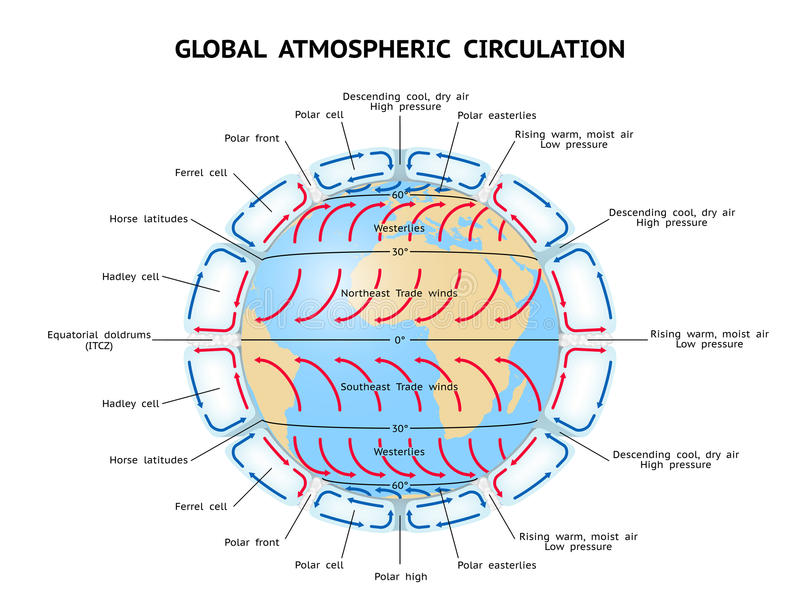
The acronym GCM originally stood for General Circulation Model, but in the present concern about Global Warming, a second meaning has come into use, namely Global Climate Model. While these do not refer to the same thing, General Circulation Models are typically the tools used for modelling climate, and hence the two terms are sometimes used interchangeably. However, the term "global climate model" is ambiguous and may refer to an integrated framework that incorporates multiple components including a general circulation model, or may refer to the general class of climate models that use a variety of means to represent the climate mathematically.
A general circulation model (GCM) is a type of climate model. It employs a mathematical model of the general circulation of a planetary atmosphere or ocean. It uses the Navier–Stokes equations on a rotating sphere with thermodynamic terms for various energy sources (radiation, latent heat). These equations are the basis for computer programs used to simulate the Earth's atmosphere or oceans. Atmospheric and oceanic GCMs (AGCM and OGCM) are key components in our understanding of climate.
Versions designed for decade to century time scale climate applications were originally created by Syukuro Manabe and Kirk Bryan at the Geophysical Fluid Dynamics Laboratory (GFDL) in Princeton, New Jersey. These models are based on the integration of a variety of fluid dynamical and chemical equations.
Part 19.1.1: Structure
Three-dimensional (more properly four-dimensional) GCMs apply discrete equations for fluid motion and integrate these forward in time. They contain parameterisations for processes such as convection that occur on scales too small to be resolved directly.
A simple general circulation model (SGCM) consists of a dynamic core that relates properties such as temperature to others such as pressure and velocity. Examples are programs that solve the primitive equations, given energy input and energy dissipation in the form of scale-dependent friction, so that atmospheric waves with the highest wavenumbers are most attenuated. Such models may be used to study atmospheric processes, but are not suitable for climate projections.
Atmospheric GCMs (AGCMs) model the atmosphere (and typically contain a land-surface model as well) using imposed sea surface temperatures (SSTs). They may include atmospheric chemistry.
A GCMs consist of a dynamical core which integrates the equations of fluid motion, typically for:
- surface pressure
- horizontal components of velocity in layers
- temperature and water vapor in layers
- radiation, split into
- solar/short wave
- terrestrial/infrared/long wave
parameters for:
- convection
- land surface processes
- albedo
- hydrology
- cloud cover
A GCM contains dynamic equations that are a function of time (typically winds, temperature, moisture, and surface pressure) together with diagnostic equations that are evaluated from them for a specific time period. As an example, pressure at any height can be diagnosed by applying the hydrostatic equation to the predicted surface pressure and the predicted values of temperature between the surface and the height of interest. Pressure is used to compute the pressure gradient force in the time-dependent equation for the winds.
Part 19.1.2: Atmospheric and Oceanic Models
OGCMs model the ocean (with fluxes from the atmosphere imposed) and may contain a sea ice model. For example, the standard resolution of HadOM3 is 1.25 degrees in latitude and longitude, with 20 vertical levels, leading to approximately 1,500,000 variables.
Atmospheric (AGCMs) and oceanic GCMs (OGCMs) can be coupled to form an atmosphere-ocean coupled general circulation model (CGCM or AOGCM). With the addition of submodels such as a sea ice model or a model for evapotranspiration over land, AOGCMs become the basis for a full climate model.
AOGCMs (e.g. HadCM3, GFDL CM2.X) combine the two submodels. They remove the need to specify fluxes across the interface of the ocean surface. These models are the basis for model predictions of future climate, such as are discussed by the IPCC. AOGCMs internalise as many processes as possible. They have been used to provide predictions at a regional scale. While the simpler models are generally susceptible to analysis and their results are easier to understand, AOGCMs may be nearly as hard to analyse as the climate itself.
The fluid equations for AGCMs are made discrete using either the finite difference method or the spectral method. For finite differences, a grid is imposed on the atmosphere. The simplest grid uses constant angular grid spacing (i.e., a latitude / longitude grid). However, non-rectangular grids (e.g., icosahedral) and grids of variable resolution are more often used.
The LMDz model can be arranged to give high resolution over any given section of the planet. HadGEM1 (and other ocean models) use an ocean grid with higher resolution in the tropics to help resolve processes believed to be important for the El Niño Southern Oscillation (ENSO).
Spectral models generally use a gaussian grid, because of the mathematics of transformation between spectral and grid-point space.
Typical AGCM resolutions are between 1 and 5 degrees in latitude or longitude: HadCM3, for example, uses 3.75 in longitude and 2.5 degrees in latitude, giving a grid of 96 by 73 points (96 x 72 for some variables); and has 19 vertical levels. This results in approximately 500,000 "basic" variables, since each grid point has four variables (u,v, T, Q), though a full count would give more (clouds; soil levels). HadGEM1 uses a grid of 1.875 degrees in longitude and 1.25 in latitude in the atmosphere; HiGEM, a high-resolution variant, uses 1.25 x 0.83 degrees respectively. These resolutions are lower than is typically used for weather forecasting. Ocean resolutions tend to be higher, for example HadCM3 has 6 ocean grid points per atmospheric grid point in the horizontal.
For a standard finite difference model, uniform gridlines converge towards the poles. This would lead to computational instabilities (see CFL condition) and so the model variables must be filtered along lines of latitude close to the poles.
Ocean models suffer from this problem too, unless a rotated grid is used in which the North Pole is shifted onto a nearby landmass. Spectral models do not suffer from this problem. Some experiments use geodesic grids and icosahedral grids, which (being more uniform) do not have pole-problems. Another approach to solving the grid spacing problem is to deform a Cartesian cube such that it covers the surface of a sphere.
Part 19.2: Global Electrical Circuit
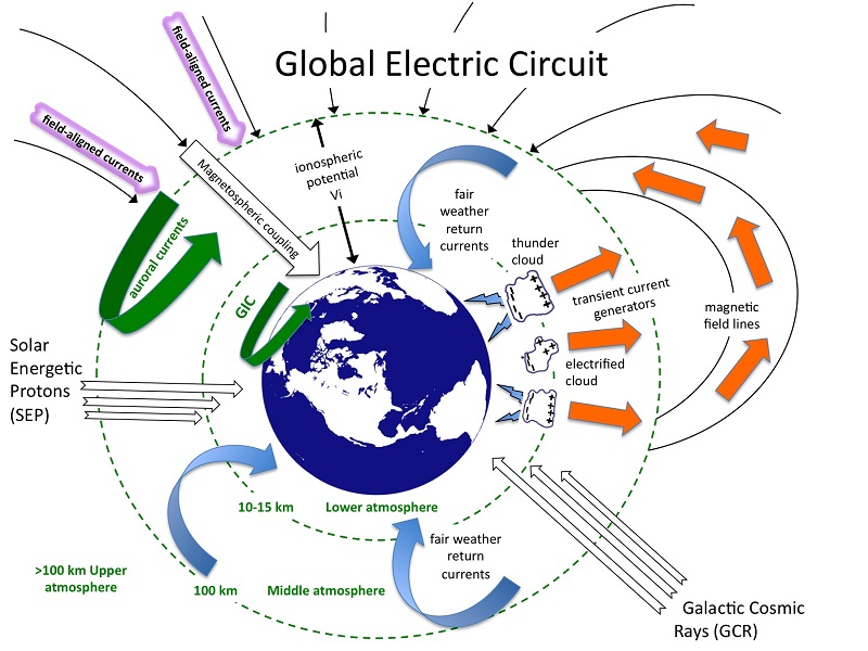
There is solid experimental evidence for the existence of electrostatic and electrodynamic links among precipitation, clouds, global temperatures, the global atmospheric electrical circuit and cosmic ray ionisation. The global circuit extends throughout the atmosphere from the planetary boundary layer to the lower layers of the ionosphere.
Cosmic rays are the principal source of atmospheric ions away from the continental boundary layer: the ions formed permit a vertical conduction current to flow in the fair weather part of the global circuit.
Through the (inverse) solar modulation of cosmic rays, the resulting columnar ionisation changes allows the global circuit to convey solar influence to meteorological phenomena of the lower atmosphere.
Electrical effects on non-thunderstorm clouds have been proposed to occur via the ion-assisted formation of ultra-fine aerosol, which can grow to sizes able to act as cloud condensation nuclei, or through the increased ice nucleation capability of charged aerosols. Even small atmospheric electrical modulations on the aerosol size distribution can affect cloud properties and modify the radiative balance of the atmosphere, through changes communicated globally by the atmospheric electrical circuit. Despite a long history of work in related areas of geophysics, the direct and inverse relationships between the global circuit and global climate remain largely quantitatively unexplored. From reviewing atmospheric electrical measurements made over two centuries and possible paleoclimate proxies, global atmospheric electrical circuit variability should be expected on many timescales.
Part 19.2.1: Atmospheric Potential Gradient
Atmospheric electricity is one of the longest-investigated geophysical topics, with a variety of measurement technologies emerging in the late eighteenth century and reliable data available from the nineteenth century. More relevant to our study of production of rain embryos through the use of negative ions is the relationship of atmospheric electricity to the global circulation systems.
Although it is well-established that clouds and aerosol modify the local atmospheric electrical parameters (Sagalyn and Faucher, 1954), aerosol microphysics simulations (Yu and Turco, 2001) and analyses of satellite-derived cloud data (Marsh and Svensmark, 2000) now suggest that aerosol formation, coagulation and in-cloud aerosol removal could themselves be influenced by changes in the electrical properties of the atmosphere (Harrison and Carslaw, 2003).
Simulations of the twentieth century climate underestimate the observed climate response to solar forcing (Stott et al., 2003), for which one possible explanation is a solar-modulated change in the atmospheric electrical potential gradient (PG) affecting clouds and therefore the radiative balance. As with many atmospheric relationships, establishing cause and effect from observations is complicated by the substantial natural variability present.
The importance of assessing the role of solar variability in climate makes it timely to review what is known about the possible relevance of the atmospheric electrical circuit of the planet to cloud formation. The scope of this section therefore includes the physical mechanisms by which global atmospheric electricity influences aerosols or clouds, negative and positive ion formation in the upper parts of the troposphereand ultimately on the electrification of rainclouds. This is not a review of thunderstorm electrification, but a discussion of the influences on the global atmospheric electrical circuit, and the atmospheric and climate processes it may influence in turn. We are specificaly interested in the interaction of negative and positive ions in the enhancement of the aerosol creation necessary to increase production of Cloud Condensation Nuclei.
Lightning strikes the earth 40,000 times per day and is the major mechanism for the stabilization of the global electrical circuits. Thunderstorms generate an electrical potential difference between the earth's surface and the ionosphere, mainly by means of lightning returning current to ground. Because of this, the ionosphere is positively charged relative to the earth. Consequently, there is always a small current of approximately 2pA per square meter transporting charged particles in the form of atmospheric ions between the ionosphere and the surface.
Fair Weather Electrodynamics: This current is carried by ions present in the atmosphere (generated mainly by cosmic rays in the free troposphere and above, and by radioactivity in the lowest 1km or so). The ions make the air weakly conductive; different locations, and meteorological conditions have different electrical conductivity. Fair weather describes the atmosphere away from thunderstorms where this weak electrical current between the ionosphere and the earth flows.
Measurement: The voltages involved in the Earth's circuit are significant. At sea level, the typical potential gradient in fair weather is 120 V/m. Nonetheless, since the conductivity of air is limited, the associated currents are also limited. A typical value is 1800 A over the entire planet. When it is not rainy or stormy, the amount of electricity within the atmosphere is typically between 1000 and 1800 amps. In fair weather, there are about 3.5 microamps per square kilometer (9 microamps per square mile). This can produce a 200+ volt difference between the head and feet of a regular person.
Carnegie curve: The Earth's electrical current varies according to a daily pattern called the Carnegie curve, caused by the regular daily variations in atmospheric electrification associated with the earth's stormy regions. The pattern also shows seasonal variation, linked to the earth's solstices and equinoxes. It was named after the Carnegie Institution for Science.
The considerable sensitivity of the planet’s albedo to cloud droplet concentrations (Twomey, 1974), presents a strong motivation for investigating possible electrical effects on cloud microphysics. Several, traditionally distinct, geophysical topics have to be considered together in order to make progress in the interdisciplinary subject area of solar-terrestrial physics, atmospheric electricity and climate.
First, the atmospheric electrical circuit has to be understood, as it communicates electrical changes globally throughout the weather-forming regions of the troposphere.
Secondly, changes in thunderstorms and shower clouds caused by surface temperature changes are likely to provide an important modulation on the global atmospheric electrical circuit.
Thirdly, the microphysics of clouds, particularly ice nucleation and water droplet formation on aerosol particles has to be assessed in terms of which mechanisms, in a myriad of other competing and complicated cloud processes, are the most likely to be significantly affected by electrical changes in the atmosphere. Changes in the global properties of clouds, even to a small extent, have implications for the long-term energy balance of the climate system: electrically-induced cloud changes present a new aspect (Kirkby, 2001).
Fourthly, galactic cosmic rays, which are modulated by solar activity, provide a major source of temporal and spatial variation in the atmosphere’s electrical properties. The cosmic ray changes include sudden reductions and perturbations on the timescales of hours (Forbush decreases and solar proton events) as well as variability on solar cycle 1(~decadal) time scales and longer. The integration of these four disparate subject areas is a major geophysical challenge, but, as this paper shows, the elements exist for an integrated quantitative understanding of the possible connections between solar changes, cosmic ray ionisation, the global atmospheric electrical circuit and climate.
The caption below summarises the geophysical processes considered in this document, which has been drawn to illustrate the links between the global atmospheric electrical circuit and the atmospheric system of precipitation.
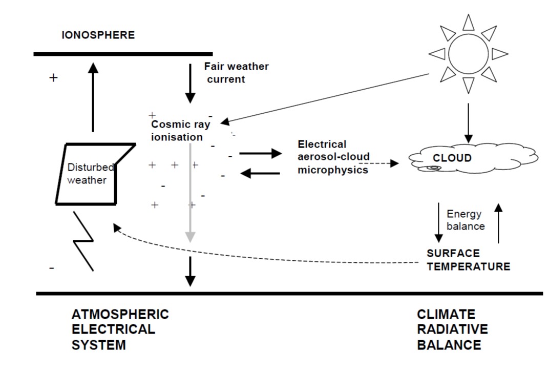
Part 19.3: Global Magnetohydrodynamic Interactions
Magnetohydrodynamics, also called magneto-fluid dynamics is the study of the magnetic properties and behaviour of electrically conducting fluids. Examples of such magnetofluids are the ionosphere, the solar corona, plasmas, liquid metals, salt water, and electrolytes. The word "magnetohydrodynamics" is derived from magneto- meaning magnetic field, hydro- meaning water, and dynamics meaning movement. The field of MHD was initiated by Hannes Alfvén.
The fundamental concept behind MHD is that magnetic fields can induce currents in a moving conductive fluid, which in turn polarizes the fluid and reciprocally changes the magnetic field itself. The set of equations that describe MHD are a combination of the Navier–Stokes equations of fluid dynamics and Maxwell’s equations of electromagnetism. These differential equations must be solved simultaneously, either analytically or numerically.
Part 19.3.1: Magnetic Reynolds Number
The magnetic Reynolds number $ {\displaystyle ( \mathrm {R}_m)} $ is the magnetic analogue of the Reynolds number used to distinguish laminer and turbulent fluid flow, a fundamental dimensionless group that occurs in magnetohydrodynamics. It gives an estimate of the relative effects of advection or induction of a magnetic field by the motion of a conducting medium, often a fluid, to magnetic diffusion. It is typically defined by: $$ {\displaystyle \mathrm {R} _{\mathrm {m} }={\frac {UL}{\eta }}~~\sim {\frac {\mathrm {induction} }{\mathrm {diffusion} }}} $$ where:
- $ {\displaystyle U } $ is a typical velocity scale of the flow,
- $ {\displaystyle L } $ is a typical length scale of the flow,
- $ {\displaystyle \eta } $ is the magnetic diffusivity.
The mechanism by which the motion of a conducting fluid generates a magnetic field is the subject of dynamo theory. When the magnetic Reynolds number is very large, however, diffusion and the dynamo are less of a concern, and in this case focus instead often rests on the influence of the magnetic field on the flow.
The simplest form of MHD, Ideal MHD, assumes that the fluid has so little resistivity that it can be treated as a perfect conductor. This is the limit of infinite magnetic Reynolds number. In ideal MHD, Lenz's law dictates that the fluid is in a sense tied to the magnetic field lines.
To explain, in ideal MHD a small rope-like volume of fluid surrounding a field line will continue to lie along a magnetic field line, even as it is twisted and distorted by fluid flows in the system. This is sometimes referred to as the magnetic field lines being "frozen" in the fluid. The connection between magnetic field lines and fluid in ideal MHD fixes the topology of the magnetic field in the fluid—for example, if a set of magnetic field lines are tied into a knot, then they will remain so as long as the fluid/plasma has negligible resistivity.
This difficulty in reconnecting magnetic field lines makes it possible to store energy by moving the fluid or the source of the magnetic field. The energy can then become available if the conditions for ideal MHD break down, allowing magnetic reconnection that releases the stored energy from the magnetic field.
In the theory of magnetohydrodynamics, the Magnetic Reynolds Number can be derived from the induction equation:
$$ {\displaystyle {\frac {\partial \mathbf {B} }{\partial t}}=\nabla \times (\mathbf {u} \times \mathbf {B} )+\eta \nabla ^{2}\mathbf {B} } $$Where
- $ {\displaystyle \mathbf {B} } $ is the magnetic field,
- $ {\displaystyle \mathbf {u} } $ is the fluid velocity,
- $ {\displaystyle \eta } $ is the magnetic diffusivity.
Part 19.3.2: The Lorentz Force
In classical electromagnetism, the Lorentz force law is used as the definition of the electric and magnetic fields $ {\displaystyle \mathbf {E} } $ and $ {\displaystyle \mathbf {B} } $ . To be specific, the Lorentz force is understood to be the following empirical statement:
The electromagnetic force $ {\displaystyle \mathbf {F} } $ on a test charge at a given point and time is a certain function of its charge $ {\displaystyle q } $ and velocity $ {\displaystyle v } $ , which can be parameterized by exactly two vectors $ {\displaystyle \mathbf {E} } $ and $ {\displaystyle \mathbf {B} } $ , in the functional form:
$$ {\displaystyle \mathbf {F} =q(\mathbf {E} +\mathbf {v} \times \mathbf {B} )} $$This is valid, even for particles approaching the speed of light. So the two vector fields $ {\displaystyle \mathbf {E} } $ and $ {\displaystyle \mathbf {B} } $ are thereby defined throughout space and time, and these are called the "electric field" and "magnetic field". The fields are defined everywhere in space and time with respect to what force a test charge would receive regardless of whether a charge is present to experience the force.
As a definition of $ {\displaystyle \mathbf {E} } $ and $ {\displaystyle \mathbf {B} } $ , the Lorentz force is only a definition in principle because a real particle (as opposed to the hypothetical "test charge" of infinitesimally-small mass and charge) would generate its own finite $ {\displaystyle \mathbf {E} } $ and $ {\displaystyle \mathbf {B} } $ fields, which would alter the electromagnetic force that it experiences. In addition, if the charge experiences acceleration, as if forced into a curved trajectory, it emits radiation that causes it to lose kinetic energy.
In general, the electric and magnetic fields are functions of the position and time. Therefore, explicitly, the Lorentz force can be written as:
$$ {\displaystyle \mathbf {F} \left(\mathbf {r} (t),{\dot {\mathbf {r} }}(t),t,q\right)=q\left[\mathbf {E} (\mathbf {r} ,t)+{\dot {\mathbf {r} }}(t)\times \mathbf {B} (\mathbf {r} ,t)\right]} $$In which $ {\displaystyle \mathbf {r} } $ is the position vector of the charged particle, $ {\displaystyle t } $ is time, and the overdot is a time derivative.
A positively charged particle will be accelerated in the same linear orientation as the $ {\displaystyle \mathbf {E} } $ field, but will curve perpendicularly to both the instantaneous velocity vector $ {\displaystyle \mathbf {v} } $ and the $ {\displaystyle \mathbf {B} } $ field according to the right-hand rule.
The term $ {\displaystyle q } $ $ {\displaystyle \mathbf {E} } $ is called the electric force, while the term $ {\displaystyle q } $ $ {\displaystyle \mathbf {(v x B)} } $ is called the magnetic force. According to some definitions, the term "Lorentz force" refers specifically to the formula for the magnetic force.
The Lorentz force is a force exerted by the electromagnetic field on the charged particle, that is, it is the rate at which linear momentum is transferred from the electromagnetic field to the particle. Associated with it is the power which is the rate at which energy is transferred from the electromagnetic field to the particle.
Part 19.3.3: Theoretical MHD
Theoretical or Ideal Magnetohydrodynamiccs: The ideal MHD equations consist of the continuity equation, the Cauchy momentum equation, Ampere's Law neglecting displacement current, and a temperature evolution equation. As with any fluid description to a kinetic system, a closure approximation must be applied to highest moment of the particle distribution equation. This is often accomplished with approximations to the heat flux through a condition of adiabaticity or isothermality.
The main quantities which characterize the electrically conducting fluid are the bulk plasma velocity field $ {\displaystyle \mathbf {v}} $ , the current density $ {\displaystyle \mathbf {J}} $ , the mass density $ {\displaystyle \rho} $ , and the plasma pressure $ {\displaystyle p} $ . The flowing electric charge in the plasma is the source of a magnetic field $ {\displaystyle \mathbf {B}} $ and electric field $ {\displaystyle \mathbf {E}} $ . All quantities generally vary with time $ {\displaystyle t} $ .
The mass continuity equation is:
$$ {\displaystyle {\frac {\partial \rho }{\partial t}}+\nabla \cdot \left(\rho \mathbf {v} \right)=0.} $$ .The Cauchy momentum equation is:
$$ {\displaystyle \rho \left({\frac {\partial }{\partial t}}+\mathbf {v} \cdot \nabla \right)\mathbf {v} =\mathbf {J} \times \mathbf {B} -\nabla p.} $$The Lorentz force term $ {\displaystyle \mathbf {J x B } } $ can be expanded using Ampère's law and the vector calculus identity:
$$ {\displaystyle {\tfrac {1}{2}}\nabla (\mathbf {B} \cdot \mathbf {B} )=(\mathbf {B} \cdot \nabla )\mathbf {B} +\mathbf {B} \times (\nabla \times \mathbf {B} )} $$To give:
$$ {\displaystyle \mathbf {J} \times \mathbf {B} ={\frac {\left(\mathbf {B} \cdot \nabla \right)\mathbf {B} }{\mu _{0}}}-\nabla \left({\frac {B^{2}}{2\mu _{0}}}\right),} $$Where the first term on the right hand side is the magnetic tension force and the second term is the magnetic pressure force.
The ideal Ohm's law for a plasma is given by:
$$ {\displaystyle \mathbf {E} +\mathbf {v} \times \mathbf {B} =0.} $$ .Faraday's law is:
$$ {\displaystyle {\frac {\partial \mathbf {B} }{\partial t}}=-\nabla \times \mathbf {E} .} $$ .The low-frequency Ampère's law neglects displacement current and is given by:
$$ {\displaystyle \mu _{0}\mathbf {J} =\nabla \times \mathbf {B} .} $$ .The magnetic divergence constraint is:
$$ {\displaystyle \nabla \cdot \mathbf {B} =0.} $$ .The energy equation is given by:
$$ {\displaystyle {\frac {\mathrm {d} }{\mathrm {d} t}}\left({\frac {p}{\rho ^{\gamma }}}\right)=0,} $$This energy equation is only applicable in the absence of shocks or heat conduction as it assumes that the entropy of a fluid element does not change.
Section Twenty: Clouds: An Overview
In meteorology, a cloud is a localized concentration of aerosols consisting of miniature liquid droplets, frozen crystals, or other particles suspended in the atmosphere of the earth. Water, and or, various other chemicals may compose the droplets and crystals. On Earth, clouds are formed as a result of saturation of the air when it is cooled to its dew point, or when it gains sufficient moisture (usually in the form of water vapor) from an adjacent source to raise the dew point to the ambient temperature.
Genus types in the troposphere have Latin names because of the universal adoption of Luke Howard's nomenclature that was formally proposed in 1802. It became the basis of a modern international system that divides clouds into five physical forms which can be further divided or classified into altitude levels to derive ten basic genera.
The main representative cloud types for each of these forms are stratiform, cumuliform, stratocumuliform, cumulonimbiform, and cirriform. Low-level clouds do not have any altitude-related prefixes. However mid-level stratiform and stratocumuliform types are given the prefix alto- while high-level variants of these same two forms carry the prefix cirro-. In both cases, strato- is dropped from the latter form to avoid double-prefixing.
Genus types with sufficient vertical extent to occupy more than one level do not carry any altitude related prefixes. They are classified formally as low- or mid-level depending on the altitude at which each initially forms, and are also more informally characterized as multi-level or vertical.
Most of the ten genera derived by this method of classification can be subdivided into species and further subdivided into varieties. Very low stratiform clouds that extend down to the Earth's surface are given the common names fog and mist, but have no Latin names.
Tropospheric clouds have a direct effect on the Global Electrical Circuit throgh their interaction with incoming solar radiation froms the sun which can contribute to a cooling effect where and when these clouds occur, or trap longer wave radiation that reflects back up from the Earth's surface which can cause a warming effect. The altitude, form, and thickness of the clouds are the main factors that affect the local heating or cooling of Earth and the atmosphere.
The importance of the water cycle, and the role clouds play in it should be self evident. Although here it is important to say that the role microphysical processes play in the water cycle is less clear. The basis for this document is to provide some thermodynamic justification for the inclusion of negative Ion as a basis for the formation of nucleation units of water in clouds or in the upper portion of the troposphere.
Cloud physics owes much of its origins to attempts, dating to the middle part of the last century, to artificially influence precipitation formation and weather. The basic idea was that by altering cloud microphysical processes it might be possible to make clouds rain more, or less effectively, thereby bringing needed rainfall to dry regions, or perhaps limiting the negative impacts of severe whether.
However, the links between cloud microphysical processes and rainfall have been a subjrct of controversy, this is in part due to the difficulties in including the turbulent aspects of vortices and interactions with the Earth's boundary layer. Hence the importance of cloud microphysical relative to cloud macrophysical processes has proven difficult to establish in any general sense. This will not be a problem for our microphysics model of negative ion water droplet creation.
Radiation is also an important reason for studying clouds. Clouds reflect significant amounts of solar radiation. As much as on an annual and global average. This is a large number, more than a factor of ten larger than the radiative forcing associated with a doubling of concentrations in the atmosphere. This tendency of clouds to reflect solar radiation warms the planet, and is called the albedo effect. or the shortwave cloud radiative effect, or sometimes simply “shortwave cloud forcing.”
This strong tendency of clouds to cool the surface is partially compensated by their greenhouse effect. By absorbing thermal radiation emitted at high temperatures (characteristic of the surface) and re-emitting it at colder temperatures (characteristic of the clouds) the net amount of thermal radiation emitted to space is reduced, thus acting to reduce the planets ability to cool itself. This is a warming, or greenhouse, effect, but can also be called the longwave cloud radiative effect, or longwave cloud radiative forcing.
Our interest in cloud physics is influenced by a desire to modify the microphysics of the local clouds so as to influence the amount of precipitation over a control area of the Earth’s ecosystem. Our invention uses the water droplet nucleation ability of negative ions to increase the density of nucleated water droplets in the upper troposphere to cause the deliberate modification of cloud thermodynamic properties to increase the number of Cloud Condensation Nuclei to initiate precipitation.
Our model will only consider the interaction of negative ions with cumuliform clouds with little vertical extent, common in the summer, that are often referred to as "fair weather clouds". These fair weather clouds generally form at lower altitudes (500–3000 m (1,500–10,000 ft)), but in hot and dry countries or over mountainous terrain these clouds can occur at an altitude of up to 6,000 m (20,000 ft). They show no significant vertical development, indicating that the temperature in the atmosphere above them either drops off very slowly or not at all with altitude; that is, the environmental lapse rate is small.
Air below the cloud base can be quite turbulent due to the thermals that formed the clouds. Our prototype ingects negative-ions into a thermal plume which rises to the cloud base to increase the aerosol nucleation rate to enhance the probability of precipitation within the footprint of our precipitation enhancement technology.
Section Twenty-One: Atmospheric Electricity
Electrical effects on Fair Weather Clouds have been proposed to occur via the ion-assisted formation of ultra-fine aerosol, which can grow to sizes able to act as cloud condensation nuclei, or through the increased ice nucleation capability of charged aerosols. Even small atmospheric electrical modulations on the aerosol size distribution can affect cloud properties and modify the local radiative balance of the planetary boundary layer of the atmosphere, through changes communicated globally by the atmospheric electrical circuit. Despite a long history of work in related areas of geophysics, the direct and inverse relationships between the global circuit and the local climate remain largely quantitatively unexplored.
Part 21.1: Atmospheric Potential Gradient
Atmospheric electricity is one of the longest-investigated geophysical topics, with a variety of measurement technologies emerging in the late eighteenth century and reliable data available from the nineteenth century. More relevant to our study of production of Cloud Condensation Nuclei through the use of negative ions as condensation units, is the relationship of atmospheric electricity at the surface of the local planetary boundary layer and its effects on local precipitation.
Although it is well-established that clouds and aerosol modify the local atmospheric electrical parameters (Sagalyn and Faucher, 1954), aerosol microphysics simulations (Yu and Turco, 2001) and analyses of satellite-derived cloud data (Marsh and Svensmark, 2000) now suggest that aerosol formation, coagulation and in-cloud aerosol removal are influenced by changes in the electrical properties of the atmosphere (Harrison and Carslaw, 2003).
The importance of assessing the role of solar variability in the production of precipitation at a local level makes it timely to review what is known about the possible relevance of the atmospheric electrical circuit of the planet to cloud formation and its relevance to the initiation of precipitation and rainfall. The scope of this chapter therefore includes the physical mechanisms by which global atmospheric electricity influences aerosols or clouds, negative and positive ion formation in the Stratosphereand ultimately on the electrification of rainclouds. This is not a review of thunderstorm electrification, but a discussion of the influences on the global atmospheric electrical circuit, and the atmospheric and precipitation processes it may influence. We are specificaly interested in the interaction of negative and positive ions in the enhancement of the aerosol creation of water droplets.
Lightning strikes the earth 40,000 times per day and is the major mechanism for the stabilization of the global electrical circuits. Thunderstorms generate an electrical potential difference between the earth's surface and the ionosphere, mainly by means of lightning returning current to ground. Because of this, the ionosphere is positively charged relative to the earth. Consequently, there is always a small current of approximately 2pA per square meter transporting charged particles in the form of atmospheric ions between the ionosphere and the surface.
Fair Weather Electrodynamics: This current is carried by ions present in the atmosphere (generated mainly by cosmic rays in the free troposphere and above, and by radioactivity in the lowest 1km or so). The ions make the air weakly conductive; different locations, and meteorological conditions have different electrical conductivity. Fair weather describes the atmosphere away from thunderstorms where this weak electrical current between the ionosphere and the earth flows.
Measurement: The voltages involved in the Earth's circuit are significant. At sea level, the typical potential gradient in fair weather is 120 V/m. Nonetheless, since the conductivity of air is limited, the associated currents are also limited. A typical value is 1800 A over the entire planet. When it is not rainy or stormy, the amount of electricity within the atmosphere is typically between 1000 and 1800 amps. In fair weather, there are about 3.5 microamps per square kilometer (9 microamps per square mile). This can produce a 200+ volt difference between the head and feet of a regular person.
Carnegie curve: The Earth's electrical current varies according to a daily pattern called the Carnegie curve, caused by the regular daily variations in atmospheric electrification associated with the earth's stormy regions. The pattern also shows seasonal variation, linked to the earth's solstices and equinoxes. It was named after the Carnegie Institution for Science.
The considerable sensitivity of the planet’s albedo to cloud droplet concentrations (Twomey, 1974), presents a strong motivation for investigating electrical effects on cloud microphysics. Several, traditionally distinct, geophysical topics have to be considered together in order to make progress in the interdisciplinary subject area of solar-terrestrial physics, atmospheric electricity and precipitation.
1. The atmospheric electrical circuit has to be understood, as it communicates electrical changes globally throughout the weather-forming regions of the troposphere.
2. Secondly, changes in thunderstorms and shower clouds caused by surface temperature changes are likely to provide an important modulation on the global atmospheric electrical circuit.
3. Thirdly, the microphysics of clouds, particularly ice nucleation and water droplet formation on aerosol particles has to be assessed in terms of which mechanisms, in a myriad of other competing and complicated cloud processes, are the most likely to be significantly affected by electrical changes in the atmosphere. Changes in the global properties of clouds, even to a small extent, have implications for the long-term energy balance of the climate system: electrically-induced cloud changes present a new aspect (Kirkby, 2001).
4. Fourthly, galactic cosmic rays, which are modulated by solar activity, provide a major source of temporal and spatial variation in the atmosphere’s electrical properties. The cosmic ray changes include sudden reductions and perturbations on the timescales of hours (Forbush decreases and solar proton events) as well as variability on solar cycle 1(~decadal) time scales and longer.
The integration of these four disparate subject areas is a major geophysical challenge, but, as this document will show, the elements exist for an integrated quantitative understanding of the possible connections between solar changes, cosmic ray ionisation, the global atmospheric electrical circuit and precipitation.
Later, in this document we will considers aspects of the global atmospheric electrical circuit, and its modulation on different timescales. We will also summarises the physics of the links between the global circuit and cloud modification, especially through ion interaction.
Observations of a sustained electrification in the fair weather atmosphere provided the motivation for the construction of the first prototype: negative-ion emitter. The sensitivity of local meteorological patterns to the local electrical parameters are the subject of this document and will also be investigated in the future. In pursuing this, electrical measurements combined with meteorological observations are expected to offer additional insights into the physical processes causing the initiation of precipitation in the Fair Weather Cloud meteorological regime.
Section Twenty-Two: Cloud Condensation Nuclei
Cloud condensation nuclei (CCNs) are small particles typically 0.2 µm, or one hundredth the size of a cloud droplet on which water vapour condenses.
In this analysis we will consider three ways in which Cloud Condensation Nuclei can be formed in the upper layer of the troposphere. The predominant method is spontaneous nucleation in supercooled water vapor. The second way is water vapor condensation on aerosols and the final method, the basis of our precipitation enhancement process, is nucleation on positive and negative ions or earosols.
Part 22.1: Spontaneous Nucleation
Water requires a non-gaseous surface to make the transition from a vapour to a liquid; this process is called condensation. In the atmosphere of Earth, this surface presents itself as tiny solid or liquid particles called CCNs.
When no CCNs are present, water vapour supercooled at about −13 °C for 5–6 hours will provide the thermodynamic environment required for water droplets to spontaneously form. (This is the basis of the cloud chamber for detecting subatomic particles). In above-freezing temperatures, the air would have to be supersaturated to around 400% before the droplets could form.
A typical raindrop is about 2 mm in diameter, a typical cloud droplet is on the order of 0.02 mm, and a typical cloud condensation nucleus (aerosol) is on the order of 0.0001 mm or 0.1 µm or greater in diameter. The number of cloud condensation nuclei in the upper stratosphere can be measured and ranges between around 100 to 1000 per cubic centimetre.There are many different types of atmospheric particulates that can act as CCN. The particles may be composed of dust or clay, soot or black carbon. The ability of these different types of particles to form cloud droplets varies according to their size and also their exact composition, as the hygroscopic properties of these different constituents are very different. This is made even more complicated by the fact that many of the chemical species may be mixed within the particles (in particular the sulfate and organic carbon). Additionally, while some particles (such as soot and minerals) do not make very good CCN, they do act as ice nuclei in colder parts of the atmosphere.
The number and type of CCNs have a profound affect on initiation of precipitation and on the amounts of precipitation.
The concept of CCN has been used in cloud seeding, which tries to encourage rainfall by seeding the air with condensation nuclei. It has further been suggested that creating such nuclei could be used for marine cloud brightening, a climate engineering technique.
Altough we are using an aerosol type of CCN enhancement it is not of the cloud seeding type. Our process is initiated in the Surface Layer of the Planetary Boundary Layer as an increase in the population of negative ions which are allowed to reach the upper part of the troposphere through an aerosol plume created on the planetary layer of the earth's planetary boundary layer. We are going to be outlining the physics of two types of negatively charged aerosols in this document: The first process is adding a negative charge to the Oxygen moleacules in the air. The second process is to spray atomized, charge water droplets. Both of these processes occur on the planetary surface and rise to the cloud layer by buoyancy and electrostatic forces.
Of the thermodynamic potentials, the Gibbs Free Energy, proves convenient for exploring supersaturation in the atmosphere. The fundamental relation expressed in terms of the Gibbs potential, $ {\displaystyle G } $ takes the form:
$$ {\displaystyle G = G(T, p, N )} $$Which, given the Gibbs-Duhem relationship, implies that for a single component system:
$$ {\displaystyle G = Sd T − V d p} $$From the main (Entropy) postulate of thermodynamics it follows that in equilibrium the thermodynamic coordinates $ {\displaystyle (T, p, N )} $ , take on values that maximize $ {\displaystyle G} $ . This maximum principle in $ {\displaystyle G} $ provides a basis for deriving the coexistence lines between two phases of a substance, in our case water. The two phase of water which we are interested in are: the water droplet (liquid) and the vapor phase (atmospheric vapor)
As a consequence of this maximum principle, thermodynamic equilibrium between the two phases requires that $ {\displaystyle g_v = g_l} $ , and in turn, that for a change in the equilibrium conditions,$ {\displaystyle \delta g_v = \delta g_l} $ . From the Gibbs-Duhem relationship we set the parameters to constrain changes in pressure and temperature,
$$ {\displaystyle (s_v − s_l )dT = (v_v − v_l )dp } $$Where thermal and mechanical equilibrium is assumed so that $ {\displaystyle T_v = T_l = T } $ , and $ {\displaystyle p_v = p_l = p } $ . Recognizing that in equilibrium $ {\displaystyle s_v = s_l = (h_v − h_l )/T = l_v} $ , leads directly to the Clapeyron equation, whose expression in the form requires one to additionally assume that the $ {\displaystyle v_l \ll v_v } $ and that the vapor behaves as an ideal gas.
It turns out that for this relationship to be useful in the study of clouds it has to be modified to account for two, in the end, decisive effects:
1. The first is that saturated surfaces are curved, and so the surface energy associated with surface tension must be accounted for.
2. The second is that the liquid phase in the atmosphere is, for reasons we shall shortly explain, almost always a solution.
These two effects compete. Surface tension effects act to require a higher vapor pressure in equilibrium, solute effects require a lower vapor pressure in equilibrium.
Heuristically these effects can be rationalized with the help of the Figure below. The left panel indicates that molecules are continuously changing phase, but that in equilibrium the rate at which particles are entering the condensed phase equals the rate at which particles are leaving the condensed phase, indicated by C and E respectively.
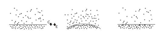
In the Figure above: Equilibrium saturation vapor pressure between a liquid and a vapor for different situations: for a surface with no surface tension effects (right) ; for a curved surface with surface tension effects (middle); over a dilute solution, where solute is shown by darkened circles (right). The motion of only some of the molecules is indicated for the purposes of illustration.
In this example the curvature of the surface and the molecular interactions of molecules in this surface layer define a distinct surface phase with a surface energy that one has to work against to expand the condensed phase. Hence a greater vapor pressure is required for particles to enter the condensed phase. Finally in the solution the depletion of the condensed phase at the phase boundary (due to the present of solute) reduces the chance of evaporation, thus in equilibrium a smaller condensation rate (and hence a smaller vapor) pressure is required to balance the reduced rate of evaporation.
Part 22.1.1: Classical Nucleation Theory
Classical nucleation theory (CNT) is the most common theoretical model used to quantitatively study the kinetics of homogeneous and hetorogeneous nucleation in the atmosphere.
Nucleation is the first step in the spontaneous formation of a new thermodynamic phase or a new structure, starting from a state of metastability. The kinetics of formation of the new phase is frequently dominated by nucleation, such that the time to nucleate determines how long it will take for the new phase to appear.
The central result of classical nucleation theory is a prediction for the rate of nucleation $ {\displaystyle R} $ , in units of (number of events)/(volume·time). For instance, a rate $ {\displaystyle R=1000\ {\text{m}}^{-3}{\text{s}}^{-1}} $ in a supersaturated vapor would correspond to an average of 1000 droplets nucleating in a volume of 1 cubic meter in 1 second.
The CNT prediction for $ {\displaystyle R} $ is: $$ {\displaystyle R\ =\ N_{S}Zj\exp \left(-{\frac {\Delta G^{*}}{k_{B}T}}\right)} $$
>where:
$ {\displaystyle \Delta G^{*}} $ is the free energy cost of the nucleus at the top of the nucleation barrier, and $ {\displaystyle k_{B}T} $ is the average thermal energy with $ {\displaystyle T} $ the absolute temperature and $ {\displaystyle k_{B}} $ the Boltzmann constant.
$ {\displaystyle N_{S}} $ is the number of nucleation sites.
$ {\displaystyle j} $ is the rate at which molecules attach to the nucleus.
$ {\displaystyle Z} $ is the Zeldovich factor, (named after Yakov Zeldovich) which gives the probability that a nucleus at the top of the barrier will go on to form the new phase, rather than dissolve.
This expression for the rate can be thought of as a product of two factors: the first, $ {\displaystyle N_{S}\exp \left(-\Delta G^{*}/k_{B}T\right)} $ , is the number of nucleation sites multiplied by the probability that a nucleus of critical size has grown around it. It can be interpreted as the average, instantaneous number of nuclei at the top of the nucleation barrier.
Free energies and probabilities are closely related. The probability of a nucleus forming at a site is proportional to $ {\displaystyle \exp[-\Delta G^{*}/kT]} $ . So if $ {\displaystyle \Delta G^{*}} $ is large and positive the probability of forming a nucleus is very low and nucleation will be slow.
The second factor in the expression for the rate is the dynamic part, $ {\displaystyle Zj} $ . Here, $ {\displaystyle j} $ expresses the rate of incoming matter and $ {\displaystyle Z} $ is the probability that a nucleus of critical size (at the maximum of the energy barrier) will continue to grow and not dissolve. The Zeldovich factor is derived by assuming that the nuclei near the top of the barrier are effectively diffusing along the radial axis. By statistical fluctuations, a nucleus at the top of the barrier can grow diffusively into a larger nucleus that will grow into a new phase, or it can lose molecules and shrink back to nothing. The probability that a given nucleus goes forward is $ {\displaystyle Z} $ .
Taking into consideration kinetic theory and assuming that there is the same transition probability in each direction, it is widely accepted that $ {\displaystyle x^{2}=2Dt} $ . As $ {\displaystyle Zj} $ determines the hopping rate, the previous formula can be rewritten in terms of the mean free path and the mean free time $ {\displaystyle \lambda ^{2}=2D\tau } $ .
Consequently, a relation of $ {\displaystyle Zj} $ in terms of the diffusion coefficient is obtained:
$$ {\displaystyle Zj={\frac {1}{\tau }}={\frac {2D}{\lambda ^{2}}}} $$ .Further considerations can be made in order to study temperature dependence. Therefore, Einstein-Stokes relation is introduced under the consideration of a spherical shape:
$$ {\displaystyle D={\frac {k_{B}T}{6\pi \eta \lambda }}} $$ .Considering the last two expressions, it is seen that $ {\displaystyle Zj} $ $ {\displaystyle \propto T} $ . If $ {\displaystyle T\approx T_{m}} $ , being $ {\displaystyle T_{m}} $ the melting temperature, the ensemble gains high velocity and makes $ {\displaystyle Zj} $ and $ {\displaystyle \Delta G^{*}} $ to increase and hence, $ {\displaystyle R} $ decreases. If $ {\displaystyle T\ll T_{m}} $ , the ensemble has a low mobility, which causes $ {\displaystyle R} $ to decrease as well.
Part 22.1.2: Homogeneous Nucleation
Homogeneous nucleation is much rarer than heterogeneous nucleation. However, homogeneous nucleation is simpler and easier to understand than heterogeneous nucleation, so the easiest way to understand heterogeneous nucleation is to start with homogeneous nucleation. So we will outline the CNT calculation for the homogeneous nucleation barrier $ {\displaystyle \Delta G^{*}} $ .
To understand if nucleation is fast or slow, $ {\displaystyle \Delta G(r)} $ , the Gibbs free energy change as a function of the size of the nucleus, needs to be calculated.
The classical theory assumes that even for a microscopic nucleus of the new phase, we can write the free energy of a droplet $ {\displaystyle \Delta G} $ as the sum of a bulk term that is proportional to the volume of the nucleus, and a surface term, that is proportional to its surface area:
$$ {\displaystyle \Delta G={\frac {4}{3}}\pi r^{3}\Delta g_{v}+4\pi r^{2}\sigma } $$The first term is the volume term, and as we are assuming that the nucleus is spherical, this is the volume of a sphere of radius $ {\displaystyle r} $ . $ {\displaystyle \Delta g_{v}} $ is the difference in free energy per unit of volume between the phase that nucleates and the thermodynamic phase nucleation is occurring in. For example, if water is nucleating in supersaturated air in the troposphere, then $ {\displaystyle \Delta g_{v}} $ is the free energy per unit of volume of water minus that of supersaturated air at the same pressure.
As nucleation only occurs when the air is supersaturated, $ {\displaystyle \Delta g_{v}} $ is always negative. The second term comes from the interface at surface of the nucleus, which is why it is proportional to the surface area of a sphere. $ {\displaystyle \sigma } $ is the surface tension of the interface between the nucleus and its surroundings, which is always positive.
For small $ {\displaystyle r} $ the second surface term dominates and $ {\displaystyle \Delta G(r)>0} $ . The free energy is the sum of an $ {\displaystyle r^{2}} $ and $ {\displaystyle r^{3}} $ terms. Now the $ {\displaystyle r^{3}} $ terms varies more rapidly with $ {\displaystyle r} $ than the $ {\displaystyle r^{2}} $ term, so as small $ {\displaystyle r} $ the $ {\displaystyle r^{2}} $ term dominates and the free energy is positive while for large $ {\displaystyle r} $ , the $ {\displaystyle r^{3}} $ term dominates and the free energy is negative. Thus at some intermediate value of $ {\displaystyle r} $ , the free energy goes through a maximum, and so the probability of formation of a nucleus goes through a minimum. There is a least-probable nucleus size, i.e., the one with the highest value of $ {\displaystyle \Delta G} $
Where:
$$ {\displaystyle \left[{\frac {dG}{dr}}\right]_{r=r_{c}}=0\implies r_{c}={\frac {2\sigma }{|\Delta g_{v}|}}} $$Addition of new molecules to nuclei larger than this critical radius, $ {\displaystyle r_{c}} $ , decreases the free energy, so these nuclei are more probable. The rate at which nucleation occurs is then limited by, i.e., determined by the probability, of forming the critical nucleus. This is just the exponential of minus the free energy of the critical nucleus $ {\displaystyle \Delta G^{*}} $ , which is:
$$ {\displaystyle \Delta G^{*}={\frac {16\pi \sigma ^{3}}{3|\Delta g_{v}|^{2}}}} $$This is the free energy barrier needed in the CNT expression for $ {\displaystyle R} $ above.
In the discussion above, we assumed the growing nucleus to be three-dimensional and spherical. Similar equations can be set up for other dimensions and/or other shapes, using the appropriate expressions for the analogues of volume and surface area of the nucleus. One will then find out that any non-spherical nucleus has a higher barrier height $ {\displaystyle \Delta G^{*}} $ than the corresponding spherical nucleus. This can be understood from the fact that a sphere has the lowest possible surface area to volume ratio, thereby minimizing the (unfavourable) surface contribution with respect to the (favourable) bulk volume contribution to the free energy. Assuming equal kinetic prefactors, the fact that $ {\displaystyle \Delta G^{*}} $ is higher for non-spherical nuclei implies that their formation rate is lower. This explains why in homogeneous nucleation usually only spherical nuclei are taken into account.
From an experimental standpoint, this theory grants tuning of the critical radius through the dependence of $ {\displaystyle \Delta G} $ on temperature. The variable $ {\displaystyle \Delta g_{v}} $ , described above, can be expressed as:
$$ {\displaystyle \Delta G={\frac {\Delta H_{f}(T_{m}-T)}{T_{m}}}\implies \Delta g_{v}={\frac {\Delta H_{f}(T_{m}-T)}{V_{at}T_{m}}}} $$Where $ {\displaystyle T_{m}} $ is the melting point and $ {\displaystyle H_{f}} $ is the enthalpy of formation for the material. Furthermore, the critical radius can be expressed as:
$$ {\displaystyle r_{c}\ =\ {\frac {2\sigma }{\Delta H_{f}}}{\frac {V_{at}T_{m}}{T_{m}-T}}\implies \Delta G^{*}={\frac {16\pi \sigma ^{3}}{3(\Delta H_{f})^{2}}}\left({\frac {V_{at}T_{m}}{T_{m}-T}}\right)^{2}} $$Revealing a dependence of reaction temperature. Thus as you increase the temperature near $ {\displaystyle T_{m}} $ , the critical radius will increase. Same happens when you move away from the melting point, the critical radius and the free energy decrease.
Part 22.1.3: Hetorogeneous Nucleation
Unlike homogeneous nucleation, heterogeneous nucleation occurs on a surface or impurity. It is much more common than homogeneous nucleation. This is because the nucleation barrier for heterogeneous nucleation is much lower than for homogeneous nucleation. To see this, note that the nucleation barrier is determined by the positive term in the free energy $ {\displaystyle \Delta G} $ , which is proportional to the total exposed surface area of a nucleus. For homogeneous nucleation the surface area is simply that of a sphere. For heterogeneous nucleation, however, the surface area is smaller since part of the nucleus boundary is accommodated by the surface or impurity onto which it is nucleating.
There are several factors which determine the precise reduction in the exposed surface area. These factors include the size of the droplet, the contact angle,$ {\displaystyle \theta } $ , between the droplet and surface, and the interactions at the three phase interfaces: liquid-solid, solid-vapor, and liquid-vapor.
The free energy needed for heterogeneous nucleation, $ {\displaystyle \Delta G^{het}} $ , is equal to the product of homogeneous nucleation, $ {\displaystyle \Delta G^{hom}} $ , and a function of the contact angle, $ {\displaystyle f(\theta )} $ :
$$ {\displaystyle \Delta G^{het}=f(\theta )\Delta G^{hom},\qquad f(\theta )={\frac {2-3\cos \theta +\cos ^{3}\theta }{4}}} $$ .Section Twenty-Three: Cloud Droplet Growth
We will be discussing two different processes by which nucleas droplets may attain radii of several microns and so form a cloud. We will discuss the diffusion of water vapour to and its condensation upon their surface, and coalescence of droplets relative to each other by virtue of Brownian Motion, small-scale turbulance, electrical forces, and differential rates of fall under gravity.
Part 23.1: Diffusional Growth
Droplet growth, or evaporation, is described by diffusional growth theory. Drops grow because they find themselves in an environment where the saturation vapor pressure exceeds the equilibrium vapor pressure at the surface of the droplet, likewise they shrink, if the saturation vapor pressure at their surface exceeds that of their environment. The vapor pressure gradient determines whether or not water vapor molecules diffuse toward, or away, from the surface of droplets.
In most instances the drop radius is much larger than the mean free path of the water vapor molecules, and it is okay to treat condensation/evaporation using a continuum description encapsulated by the theory of diffusion. For very small droplets or haze particles it may become necessary to consider kinetic effects, i.e.,the statistics of molecular interactions described by the kinetic theory of gases, so as to modify the standard diffusion-based description.
The starting point for the standard description of diffusional growth is Ficks First Law.
Part 23.1.1: Fick's first law for gases
Fick's first law for binary gas mixtures is outlined below.
We assume: thermal diffusion is negligible; the body force per unit mass is the same on both species; and either pressure is constant or both species have the same molar mass. Under these conditions the kinetic theory of gases reduces to this version of Fick's law:
$$ {\displaystyle \mathbf {V_{i}} =-D\,\nabla \ln y_{i} \,\,\,\,\,\,\,\,\,\,\,\,\,\,\,(23.1.1.1)} $$Where $ {\displaystyle \mathbf {V_{i}}} $ is the diffusion velocity of species $ {\displaystyle \mathbf i} $ . In terms of species flux this is:
$$ {\displaystyle \mathbf {J_{i}} =-{\frac {\rho D}{M_{i}}} \nabla y_{i}\,\,\,\,\,\,\,\,\,\,\,\,\,\,\,(23.1.1.2)} $$If, additionally, $ {\displaystyle \nabla \rho =0} $ , this reduces to the most common form of Fick's law:
$$ {\displaystyle \mathbf {J_{i}} =-D\nabla \varphi \,\,\,\,\,\,\,\,\,\,\,\,\,\,\,(23.1.1.3) } $$If (instead of or in addition to $ {\displaystyle \nabla \rho =0} $ ) both species have the same molar mass, Fick's law becomes:
$$ {\displaystyle \mathbf {J_{i}} =-{\frac {\rho D}{M_{i}}}\nabla x_{i} \,\,\,\,\,\,\,\,\,\,\,\,\,\,\,(23.1.1.4)} $$Where $ {\displaystyle x_{i}} $ is the mole fraction of species $ i $ .
Part 23.1.2: Fick's Second Law for Gases
Fick's second law can be derived from Fick's first law and the mass conservation in absence of any chemical reactions: $$ {\displaystyle {\frac {\partial \varphi }{\partial t}}+{\frac {\partial }{\partial x}}J=0\Rightarrow {\frac {\partial \varphi }{\partial t}}-{\frac {\partial }{\partial x}}\left(D{\frac {\partial }{\partial x}}\varphi \right)\,=0 \,\,\,\,\,\,\,\,\,\,\,\,\,\,\,(23.1.2.1)} $$
Assuming the diffusion coefficient span class="math display">$ {\displaystyle D} $ to be a constant, one can exchange the orders of the differentiation and multiply by the constant:
$$ {\displaystyle {\frac {\partial }{\partial x}}\left(D{\frac {\partial }{\partial x}}\varphi \right)=D{\frac {\partial }{\partial x}}{\frac {\partial }{\partial x}}\varphi =D{\frac {\partial ^{2}\varphi }{\partial x^{2}}} \,\,\,\,\,\,\,\,\,\,\,\,\,\,\,(23.1.2.2)} $$Thus, receive the form of the Fick's equations as was stated above.
For the case of diffusion in two or more dimensions Fick's second law becomes:
$$ {\displaystyle {\frac {\partial \varphi }{\partial t}}=D\,\nabla ^{2}\varphi \,\,\,\,\,\,\,\,\,\,\,\,\,\,\,(23.1.2.3)} $$Which is analogous to the heat equation.
If the diffusion coefficient is not a constant, but depends upon the coordinate or concentration, Fick's second law yields:
$$ {\displaystyle {\frac {\partial \varphi }{\partial t}}=\nabla \cdot (D\,\nabla \varphi ) \,\,\,\,\,\,\,\,\,\,\,\,\,\,\,(23.1.2.4)} $$The equation above applies when the diffusion coefficient is isotropic; in the case of anisotropic diffusion, D is a symmetric positive definite matrix, and the equation is written (for three dimensional diffusion) as:
$$ {\displaystyle {\frac {\partial \phi (\mathbf {r} ,t)}{\partial t}}=\sum _{i=1}^{3}\sum _{j=1}^{3}{\frac {\partial }{\partial x_{i}}}\left[D_{ij}(\phi ,\mathbf {r} ){\frac {\partial \phi (\mathbf {r} ,t)}{\partial x_{j}}}\right] \,\,\,\,\,\,\,\,\,\,\,\,\,\,\,(23.1.2.5)} $$Part 23.2: Growth of Single Droplet by Condensation
The following argument can be found in The Physics of Clouds, Second Edition, by B.J. Mason
We begin our discussion by considering an isolated water droplet of mass $ {\displaystyle m,} $ radius $ {\displaystyle r} $ and density $ {\displaystyle \rho_L} $ to be stationary relative to a macroscopic area of the atmosphere, so that we do not have to worry about boundary effects. Our droplet is growing very slowly by the diffusion of water vapour to its surface.
If the temperature and vapor density in a large volume surrounding our droplet remain constant, a steady-state diffusion process will be established around the droplet so that the mass of water vapour diffusing across any spherical surface of radius $ {\displaystyle R} $ centered on the droplet will be independent of $ {\displaystyle R} $ and time. The flux of water vapour towards the droplet will then be given by Fick's Law of diffusion and is:
$$ {\displaystyle F = {\frac{\mathbf {d} m}{\mathbf {d} t}} = {4 \pi R^2 D} \frac{\mathbf {d} \rho}{\mathbf {d} R} = Constant (B) } $$Where $ {\displaystyle{\frac{\mathbf {d} m}{\mathbf {d} t}}} $ is the rate of increase of the droplet mass, $ {\displaystyle \frac{\mathbf {d} \rho}{\mathbf {d} R}} $ is the radial gradient of vapour density, and $ {\displaystyle D} $ is the diffusion coefficient of water vapour in air.
Integration of this equation with respect to distance from the surface of the drop where the vapour density is $ {\displaystyle \rho_r} $ to infinity where it is $ {\displaystyle \rho} $ , we have:
$$ {\displaystyle 4 \pi D \int _{\rho }^{\rho^r }d\rho = \int _{\infty }^{r} \frac {B}{R^2} d R } $$Or $ {\displaystyle \,\,\,\,\,\,\,\,\,\,\,\,\,\,\,\,\,\,\,\,\,\,\, 4 \pi D (\rho_r - \rho) = -\frac {B}{r} = -\frac {1}{r} \frac {dm}{dt}} $ ,
and therefore: $ {\displaystyle \,\,\,\,\,\,\,\,\,\,\,\,\,\,\,\,\,\,\,\,\,\,\, \frac {dm}{dt} = 4 \pi D (\rho - \rho_r)} $ .
Condensation of water vapour on the droplet releases latent heat at a rate of $ {\displaystyle L (\frac {dm}{dt})} $ where $ {\displaystyle L} $ is the latent heat of condensation, and this is dissipated mainly by conduction through the surrounding air.
Using the same technique for the conduction of heat away from the droplet surface we get:
$$ {\displaystyle L \frac{\mathbf {d} m}{\mathbf {d} t} = -{4 \pi R^2 K \frac{dT} {dR} }} $$Where the temperature gradient $ {\displaystyle \frac{dT} {dR} } $ is negative because the temperature decreases with increasing distance from the droplet. Note that $ {\displaystyle K } $ is the thermal conductivity of the air. Integration of this equation leads us to the following:
$$ {\displaystyle L \frac{\mathbf {d} m}{\mathbf {d} t} = -L 4 \pi R^2 \rho_L \frac{dr} {dt} = 4 \pi K r (T_r - T )} $$Where $ {\displaystyle T_r} $ is the surface temperature of the drop and $ {\displaystyle T} $ is the temperature of the distant environment.
Since the saturation vapour pressure and the temperature dependence are given by:
$ {\displaystyle p_s = \rho_s R T/M } $ and $ {\displaystyle 1/p_s dp_s/dT = LM/ \mathbf {R} T^2 } $ :
$$ {\displaystyle \frac{d \rho_s} {\rho_s} = \frac {L M} {\mathbf {R}} \frac {d T} {T^2} - \frac{d T} {T }} $$Where $ {\displaystyle M} $ is the moleacular weight of water and $ {\displaystyle \mathbf {R}} $ is the universal gas constant. Integration of this equation from the surface of the drop to infinity yeilds:
$$ {\displaystyle ln \frac{\rho_s (T_r)} {\rho_s(T)} = \frac {L M} {\mathbf {R}} \frac {T_r - T} {T T_r} - ln \frac{T_r} {T} = \left ( \frac {LM - \mathbf {R} T} {\mathbf {R} T^2} \right ) ( T_r - T ) } $$Since $ {\displaystyle T_r \approxeq T} $ , therefore we can write:
$$ {\displaystyle \frac{ \rho_s (T_r)} {\rho_s(T)} = 1 + \left (\frac {L M - \mathbf {R} T} {\mathbf {R} T^2} \right)(T_r - T) + \frac {1} {2} \left ( \frac {LM - \mathbf {R} T} {\mathbf {R} T^2} \right )^2 ( T_r - T )^2 } $$Because, in most practical cases, $ {\displaystyle (T_r - T) \leq 1^o C} $ , the last term in the last equation above may be neglected, and substitution from already derived equation yields the following result:
$$ {\displaystyle \frac{ \rho_s (T_r) -\rho_s(T)} {\rho_s(T)} = \left (\frac {L M} {\mathbf {R} T} - 1 \right) \left ( \frac {T_r - T} {T} \right) = \frac {L} {4 \pi K_r T} \left ( \frac {LM } {\mathbf {R} T} - 1 \right ) \frac {dm} {dt}} $$Dividing:
$$ {\displaystyle 4 \pi D \int _{\rho }^{\rho^r }d\rho = \int _{\infty }^{r} \frac {B}{R^2} d R } $$By $ {\displaystyle \rho_s (T) } $ and add the result to the equation above yeilds:
$$ {\displaystyle { \frac{ \rho -\rho_s(T)} {\rho_s(T)} = \left( \frac {L} {4 \pi K_r T } \left( \frac {L M} {\mathbf {R} T} - 1 \right) + \frac {1} {4 \pi D_r \rho_s(T)} \right) \frac {dm} {dt}}} $$Or:
$$ {\displaystyle \frac {dm} {dt} = {\frac {4 \pi r (\rho_s / \rho_{s(T)} -1)} {\left( \frac {L}{KT} \left( \frac {LM}{\mathbf {R} T} -1 \right) + \frac {1} {D_{\rho_{s(T)}}}\right)}}} $$Or:
$$ {\displaystyle r \frac {dr} {dt} = \frac {S -1} {\left( \frac {L \rho_L}{KT} \left( \frac {LM}{\mathbf {R} T} -1 \right) + \frac {\mathbf {R} T \rho_L} {DMp_s(T)} \right)}} $$Where $ {\displaystyle S-1} $ is the supersaturation of the vapour. From this last equation describing the growth of a drop of pure water that is large enough for the curvature of the surface to have a negligeable effect and since Where $ {\displaystyle \rho_s(T_r)/ \rho_s(T)} $ is very close to unity for a drop growing at a normal rate:
$$ {\displaystyle r \frac {dr} {dt} \approxeq {\frac {(S -1)-2 \sigma_{LV}M / \rho_L \mathbf {R}T_r + i m M/ \frac {4}{3} \pi r^3 \rho_L W} {\left[ \frac {L \rho_L}{KT} \left( \frac {LM}{\mathbf {R} T} -1 \right) + \frac {\mathbf {R} T \rho_L} {DMp_s(T)}\right]}}} $$The growth of droplets by condensation may be calculated from this equation if the properties $ {\displaystyle m} $ and $ {\displaystyle W,} $ of the nucleus, the supersaturation, the temperature and pressure of the air are all specified.
Part 23.3: Growth of a population of Droplet by Condensation
Now we are ready to consider the growth of a population of droplets leading to the formation of a cloud. Having specified the initial temperature, pressure, humidity, and nucleus content of the air, the problem is then defined by four differential equations expressing the rate of change of supersaturation, temperature, droplet radius and liquid water content. The following treatment can be found in Mason and also a close treatment can be found in Jacobson (Fundamental of Atmospheric Modeling).
The supersaturation of an air mass can be expressed in terms of the difference between its dew point, $ {\displaystyle T_d} $ , and the actual temperature $ {\displaystyle T} $ , of the air. If saturated air at temperature $ {\displaystyle T} $ and vapor pressure $ {\displaystyle p_s} $ is warmed to $ {\displaystyle T + dT} $ , then the incremental increase in vapour pressure, $ {\displaystyle dp_s} $ , required to keep it saturated is given by $ {\displaystyle dp_s = \epsilon L dT/\mathbf {R}_d T^2,} $ where $ {\displaystyle L} $ is the latent heat of condensation of water vapour, $ {\displaystyle \epsilon} $ is the specific gravity of water vapour relative to that of dry air, and:
$$ {\displaystyle \mathbf {R}_d = 2.87 x {10}^6 erg g^{-1} K^{-1} } $$Is the gas constant for dry air. If now the air is still saturated while being warmed to a slightly higher temperature, $ {\displaystyle T + dT_d} $ , and therefore cooled to $ {\displaystyle T + dT} $ without condensation occuring the vapour pressure will now be in excess of saturation by an amount $ {\displaystyle dp} $ such that the supersaturation $ {\displaystyle d\sigma} $ may be written as:
$$ {\displaystyle d\sigma = \frac {dp}{p_s} = \frac {\epsilon L}{\mathbf {R}_d T^2} (dT_d - dT) \,\,\,\,\,\,\,\,\,\,\,\,\,\,\,\,\,\,\,\,\,\,\,(23.3.1) } $$ ,This formula is only valid for small changes in supersaturation.
Now the change in temperature of the air following a vertical displacement $ {\displaystyle dz} $ is given by:
$$ {\displaystyle dT = \left(\frac {-g dz}{c_p} - \frac {L d x} {c_p} \right) \,\,\,\,\,\,\,\,\,\,\,\,\,\,\,\,\,\,\,\,\,\,\,(23.3.2) } $$ ,With $ {\displaystyle g/c_p} $ being the dry air adiabatic lapse rate, $ {\displaystyle dx} $ the change in the humidity mixing ratio and $ {\displaystyle c_p} $ the specific heat of air at constant pressure. Thus we have:
$$ {\displaystyle d\sigma = \frac {\epsilon L}{\mathbf {R}_d T^2} \left( dT_d + \frac {g}{c_p}dz + \frac {L dx}{c_p} \right) \,\,\,\,\,\,\,\,\,\,\,\,\,\,\,\,\,\,\,\,\,\,\,(23.3.3) } $$ ,We may also use the following relations to represent changes occuring in slightly supersaturated dry air: $$ {\displaystyle dx + d\omega = 0 \,\,\,\,\,\,\,\,\,\,\,\,\,\,\,\,\,\,\,\,\,\,\,(23.3.4) } $$ ,
Where $ {\displaystyle \omega} $ is the liquid-water mixing ration in grams per gram of dry air.
$$ {\displaystyle \mathrm {d}x = \epsilon \mathrm {d} \left(\frac{p_s}{P}\right) = \frac {\epsilon}{P^2} (Pdp_s - p_s dP) \,\,\,\,\,\,\,\,\,\,\,\,\,\,\,\,\,\,\,\,\,\,\,(23.3.5) } $$ , $$ {\displaystyle \frac{1} {p^2}\frac{\mathrm {d}p_s}{\mathrm {d}T} = \frac {\epsilon L}{\mathbf {R}_d T^2} \,\,\,\,\,\,\,\,\,\,\,\,\,\,\,\,\,\,\,\,\,\,\,(23.3.6) } $$ , $$ {\displaystyle \frac{\mathrm {d}P}{\mathrm {d}z} = \frac {g P}{\mathbf {R}_d T} \,\,\,\,\,\,\,\,\,\,\,\,\,\,\,\,\,\,\,\,\,\,\,(23.3.7) } $$ ,Where $ {\displaystyle P} $ is the total pressure and $ {\displaystyle g} $ is the acceleration due to gravity.
Substitution from (23.3.6) and (23.3.7) into (23.3.5) gives:
$$ {\displaystyle \mathrm {d}x = -\mathrm {d} \omega = \frac {\epsilon}{P^2} \left(\frac{p_s g P}{\mathbf {R}_d T} \mathrm{d}z + \frac{\epsilon P L p_s}{\mathbf {R}_d T^2 } \mathrm {d} T_d \right)\,\,\,\,\,\,\,\,\,\,\,\,\,\,\,\,\,\,\,\,\,\,\,(23.3.8) } $$ ,and finally, substituting for $ {\displaystyle T_d} $ from (23.3.8) into (23.3.7) we get:
$$ {\displaystyle \mathrm{d} o = \frac{\epsilon L}{\mathbf{R}_d T^2} \left[g \left( \frac{1}{c_p} - \frac{T}{L \epsilon} \right)\mathrm{d} z - \left( \frac{L}{c_p} + \frac{P \mathbf{R}_d T^2}{L {\epsilon}^2 p_s} \right) \mathrm {d} \omega \right]\,\,\,\,\,\,\,\,\,\,\,\,\,\,\,\,\,\,\,\,\,\,\,(23.3.9) }.$$Then we assume that the cloud droplets are being carried up in an updraught of velocity $ {\displaystyle U} $ then equation (23.3.9) gives us an expression for the time variation of the supersaturation:
$$ {\displaystyle \frac {\mathrm{d}\sigma}{\mathrm{d}t} = AU - B \frac{\mathrm{d}\omega}{\mathrm{d} t} \,\,\,\,\,\,\,\,\,\,\,\,\,\,\,\,\,\,\,\,\,\,\,(23.3.10) } $$ ,Where: $ {\displaystyle A \, = \left(\frac {\epsilon L g}{c_p \mathrm{R}_d T^2} - \frac{g}{\mathrm{R}_d T} \right) = \frac {3.42\, \mathrm{x}\, 10^{-4}}{T} \left(2.6 \frac{L}{T} -1 \right)} $
$ {\displaystyle L }$ being measured in cal $ {\displaystyle g^{-1}} $ , and:
$$ {\displaystyle B \, = \left(\frac {\epsilon L^2}{c_p \mathrm{R}_d T^2} + \frac{P}{\epsilon p_s} \right) = \left(37.8 \frac {L^2}{T^2}\, +\, 1.62\, \frac{P}{p_s} \right)} $$The time variation of the temperature is given by substituting for $ {\displaystyle \mathrm{d} x } $ from (15.3.8) into (15.3.2) to obtain:
$$ {\displaystyle \frac { \mathrm{d}T}{\mathrm{d}t} = \frac {-g U}{c_p} \left(1 + \frac {L \epsilon p_s} {\mathrm{R}_d PT} \right)/ \left(1 + \frac{\epsilon^2 L^2 p_s}{c_p \mathrm{R}_d P T^2} \right) \,\,\,\,\,\,\,\,\,\,\,\,\,\,\,\,\,\,\,\,\,\,\,(23.3.11) } $$ ,Equation (15.3.11) expresses the fact that the supersaturation is determined by the rate at which water vapour is released for condensation by lifting and cooling of the air minus the rate at which it is condensed on the existing droplets.
The liquid-water mixing ratio is given by:
$$ {\displaystyle \frac{\mathrm {d}\omega}{\mathrm {d}t} = \frac {4}{3} \pi \frac{\rho_L}{\rho_a} \frac{\mathrm{d}}{\mathrm{d}t} \sum^r n r^3 \,\,\,\,\,\,\,\,\,\,\,\,\,\,\,\,\,\,\,\,\,\,\,(23.3.12) } $$ ,Where $ {\displaystyle n} $ is the number of droplets per $ {\displaystyle cm^3} $ of radius $ {\displaystyle r} $ and $ {\displaystyle \rho_a} $ is the air density.
If the initial conditions at the cloud base are specified then these equations may be integrated numerically to give the drop size, supersaturation, temperature, and liquid-vapour content in the cloud as a function of time and the corresponding height above cloud base.
Part 23.4: Electrical Effects on Cloud Microphysics
There is a considerable variety in the sizes and abundance of aerosol particles, ice crystals and cloud droplets present in the atmosphere. The typical molecular cluster comprising an atmospheric small ion will have a diameter of less than one nanometre.
Aerosols have diameters from 3nm to 10μm, and cloud and raindrops have diameters from 10μm to 1mm. The complexity of cloud microphysical processes results from both the different particle sizes and compositions in atmospheric clouds, and the phase changes between solid and liquid (Mason, 1971; Pruppacher and Klett, 1997).
Aerosol electrification in the atmosphere occurs from ion-aerosol attachment, facilitated by ion transport in electric fields (Pauthenier, 1956), by diffusion (Gunn 1955; Fuchs, 1963; Bricard, 1965; Boisdron and Brock, 1970). Chemical and dipole asymmetries in the ion properties generally result in a charge distribution on the aerosol, which, although the distribution may have a small mean charge, does not preclude the existence of transiently highly charged particles within the ensemble.
In the special case of radioactive aerosols, the charge arises from a competition between the self-generation of charge within the particle, and ions diffusing to the particle (Clement and Harrison,1992; Gensdarmes et al., 2001). The aerosol charge distribution can affect aerosol coagulation rates (Clement et al., 1995), which in turn may modify the particle size distribution.
In the first case, atmospheric effects would occur through changes in ion production, leading in turn to changes in aerosol nucleation, ion-aerosol attachment rates, aerosol charge equilibration times and aerosol coagulation rates, ultimately modifying clouds.
Direct evidence for the growth of ions in humid air with low aerosol content has been reported from natural radioactivity (Wilkening,1985), where ion complexes having mobilities considerably smaller than atmospheric small ions have been observed. Decrease in ion mobility results from an increase in ion size.
In the second case listed above, the electric fields caused by the global circuit could affect aerosol charging by modifying the ion environment on the boundaries of clouds where ion concentrations are profoundly asymmetric and the electric fields are enhanced (Carslaw et al., 2002). The global circuit could therefore act to communicate cosmic ray changes throughout the atmosphere, by changes in the conduction current.
Section Twenty-Four: Microphysics of Planetary Boundary Layer (PBL)
Part 24.1: Introduction
The lower part of the planetary boundary layer is that portion of the atmosphere connected to the earth boundary layer. It is in this lower section of the boundary layer that our prototypes create negative ions and we therefore need to discuss the existance and relevence of the planetary boundary layer.
The planetary boundary layer is that portion of the atmosphere in which the flow field is strongly influenced directly by interaction with the surface of the earth. Ultimately this interaction depends on molecular viscosity. It is, however, only within a few millimeters of the surface, where vertical shears are very intense, that molecular diffusion is comparable to other terms in the momentum equation.
Outside this viscous sublayer molecular diffusion is not important in the boundary layer equations for the mean wind, although it is still important for small-scale turbulent eddies. However, viscosity still has an important indirect role; it causes the velocity to vanish at the surface. As a consequence of this no-slip boundary condition, even a fairly weak wind will cause a large-velocity shear near the surface, which continually leads to the development of turbulent eddies.
These turbulent motions have spatial and temporal variations at scales much smaller than those resolved by the meteorological observing network. Such shear-induced eddies, together with convective eddies caused by surface heating, are very effective in transferring momentum to the surface and transferring heat (latent and sensible) away from the surface at rates many orders of magnitude faster than can be done by molecular processes.
Typically, due to aerodynamic drag, there is a wind gradient in the wind flow ~100 meters above the Earth's surface—the surface layer of the planetary boundary layer. Wind speed increases with increasing height above the ground, starting from zero due to the no-slip condition. Flow near the surface encounters obstacles that reduce the wind speed, and introduce random vertical and horizontal velocity components at right angles to the main direction of flow. This turbulence causes vertical mixing between the air moving horizontally at one level and the air at those levels immediately above and below it, which is important in dispersion of pollutants and in soil erosion.The presence of turbulence in the lower portions of the planetary boundary laayer is our avenue for the injection of negative ions into the upper atmosphere at the surface of the earth.
The reduction in velocity near the surface is a function of surface roughness, so wind velocity profiles are quite different for different terrain types.[5] Rough, irregular ground, and man-made obstructions on the ground can reduce the geostrophic wind speed by 40% to 50%. Over open water or ice, the reduction may be only 20% to 30%. These effects are taken into account when siting wind turbines.
For engineering purposes, the wind gradient is modeled as a simple shear exhibiting a vertical velocity profile varying according to a power law with a constant exponential coefficient based on surface type. The height above ground where surface friction has a negligible effect on wind speed is called the "gradient height" and the wind speed above this height is assumed to be a constant called the "gradient wind speed".
Part 24.2: Convective Planetary Boundary Layer
The convective planetary boundary layer (CPBL), also known as the daytime planetary boundary layer, is the part of the lower troposphere most directly affected by solar heating of the earth's surface.
This layer extends from the earth surface to a capping inversion that typically locates at a height of 1–2 km by midafternoon over land. Below the capping inversion (10-60% of CBL depth, also called entrainment zone in the daytime), CBL is divided into two sub-layers: mixed layer (35-80% of CBL depth) and surface layer (5-10% of CBL depth). The mixed layer, the major part of CBL, has a nearly constant distribution of quantities such as potential temperature, wind speed, moisture and pollutant concentration because of strong buoyancy generated convective turbulent mixing.
Parameterization of turbulent transport is used to simulate the vertical profiles and temporal variation of quantities of interest, because of the randomness and the unknown physics of turbulence.
However, turbulence in the mixed layer is not completely random, but is often organized into identifiable structures such as thermals and plumes in the CBL. Simulation of these large eddies is quite different from simulation of smaller eddies generated by local shears in the surface layer. Non-local property of the large eddies should be accounted for in the parameterization.
Part 24.3: Atmospheric Turbulence
Turbulent flow contains irregular quasi-random motions spanning a continuous spectrum of spatial and temporal scales. Such eddies cause nearby air parcels to drift apart and thus mix properties such as momentum and potential temperature across the boundary layer. Unlike the large-scale rotational flows discussed in earlier chapters, which have depth scales that are small compared to their horizontal scales, the turbulent eddies of concern in the planetary boundary layer tend to have similar scales in the horizontal and vertical. The turbulent eddies created by the corona discharge into the lower layer of the planetary boundary layer have a significant impact on the thermodynamics and the hydrodynamics of the negative ion plume.
The maximum eddy length scale is thus limited by the boundary layer depth to be about 10 3 m. The minimum length scale $ {\displaystyle (10^{-3} m) } $ is that of the smallest eddies that can exist in the presence of diffusion by molecular friction.
Even when observations are taken with very short temporal and spatial separations, a turbulent flow will always have scales that are unresolvable because they have frequencies greater than the observation frequency and spatial scales smaller than the scale of separation of the observations.
Outside the boundary layer, in the free atmosphere, the problem of unresolved scales of motion is usually not a serious one for the diagnosis or forecasting of synoptic and larger scale circulation. The eddies that contain the bulk of the energy in the free atmosphere are resolved by the synoptic network.
However, in the boundary layer, unresolved turbulent eddies are of critical importance. Through their transport of heat and moisture away from the surface they maintain the surface energy balance, and through their transport of momentum to the surface they maintain the momentum balance. The latter process dramatically alters the momentum balance of the large-scale flow in the boundary layer so that geostrophic balance is no longer an adequate approximation to the large-scale wind field. It is this aspect of boundary layer dynamics that is of primary importance for dynamical meteorology.
Part 24.4: The Boussinesq Approximation
In Planetary boundary layer fluid dynamics, the Boussinesq approximation is used in the field of buoyancy-driven flow (also known as natural convection). It ignores density differences except where they appear in terms multiplied by g, the acceleration due to gravity. The essence of the Boussinesq approximation is that the difference in inertia is negligible but gravity is sufficiently strong to make the specific weight appreciably different between the two fluids.
Boussinesq flows are common in nature (such as atmospheric fronts, oceanic circulation, katabatic winds), industry (dense gas dispersion, fume cupboard ventilation). The approximation is extremely accurate for many such flows, and makes the mathematics and physics simpler.
The Boussinesq approximation is applied to problems where the fluid varies in temperature from one place to another, driving a flow of fluid and heat transfer. The fluid satisfies conservation of mass, conservation of momentum and conservation of energy. In the Boussinesq approximation, variations in fluid properties other than density $ {\displaystyle \rho } $ are ignored, and density only appears when it is multiplied by $ {\displaystyle g } $ , the gravitational acceleration. If $ {\displaystyle u } $ is the local velocity of a parcel of fluid, the continuity equation for conservation of mass is:
$$ {\displaystyle {\frac {\partial \rho }{\partial t}}+\nabla \cdot \left(\rho \mathbf {u} \right)=0.} $$ .If density variations are ignored, this reduces to:
$$ {\displaystyle \nabla \cdot \mathbf {u} =0.} $$ .The general expression for conservation of momentum of an incompressible, Newtonian fluid (the Navier–Stokes equations) is:
$$ {\displaystyle {\frac {\partial \mathbf {u} }{\partial t}}+\left(\mathbf {u} \cdot \nabla \right)\mathbf {u} =-{\frac {1}{\rho }}\nabla p+\nu \nabla ^{2}\mathbf {u} +{\frac {1}{\rho }}\mathbf {F} ,} $$where $ {\displaystyle \nu } $ is the kinematic viscosity and $ {\displaystyle F } $ is the sum of any body forces such as gravity. In this equation, density variations are assumed to have a fixed part and another part that has a linear dependence on temperature:
$$ {\displaystyle \rho =\rho _{0}-\alpha \rho _{0}(T-T_{0}),} $$Where $ {\displaystyle \alpha } $ is the coefficient of thermal expansion. The Boussinesq approximation states that the density variation is only important in the buoyancy term.
If $ {\displaystyle F=\rho \mathbf {g} } $ is the gravitational body force, the resulting conservation equation is:
$$ {\displaystyle {\frac {\partial \mathbf {u} }{\partial t}}+\left(\mathbf {u} \cdot \nabla \right)\mathbf {u} =-{\frac {1}{\rho _{0}}}\nabla (p-\rho _{0}\mathbf {g} \cdot \mathbf {z} )+\nu \nabla ^{2}\mathbf {u} -\mathbf {g} \alpha (T-T_{0}).} $$In the equation for heat flow in a temperature gradient, the heat capacity per unit volume, $ {\displaystyle \rho C_{p}} $ , is assumed constant and the dissipation term is ignored. The resulting equation is:
$$ {\displaystyle {\frac {\partial T}{\partial t}}+\mathbf {u} \cdot \nabla T={\frac {k}{\rho C_{p}}}\nabla ^{2}T+{\frac {J}{\rho C_{p}}},} $$Where $ {\displaystyle J } $ is the rate per unit volume of internal heat production and $ {\displaystyle k } $ is the thermal conductivity.
Part 24.5: Reynolds Averaging
The Reynolds-averaged Navier–Stokes equations are time-averaged equations of motion for fluid flow. The idea behind the equations is Reynolds decomposition, whereby an instantaneous quantity is decomposed into its time-averaged and fluctuating quantities.
The RANS equations are primarily used to describe turbulent flows. These equations can be used with approximations based on knowledge of the properties of flow turbulence to give approximate time-averaged solutions to the Navier–Stokes equations. For a stationary flow of an incompressible Newtonian fluid, these equations can be written in Einstein notation in Cartesian coordinates as:
$$ {\displaystyle \rho {\bar {u}}_{j}{\frac {\partial {\bar {u}}_{i}}{\partial x_{j}}}=\rho {\bar {f}}_{i}+{\frac {\partial }{\partial x_{j}}}\left[-{\bar {p}}\delta _{ij}+\mu \left({\frac {\partial {\bar {u}}_{i}}{\partial x_{j}}}+{\frac {\partial {\bar {u}}_{j}}{\partial x_{i}}}\right)-\rho {\overline {u_{i}^{\prime }u_{j}^{\prime }}}\right].} $$The left hand side of this equation represents the change in mean momentum of a fluid element owing to the unsteadiness in the mean flow and the convection by the mean flow. This change is balanced by the mean body force, the isotropic stress owing to the mean pressure field, the viscous stresses, and apparent stress $ {\displaystyle \left(-\rho {\overline {u_{i}^{\prime }u_{j}^{\prime }}}\right)} $ owing to the fluctuating velocity field, generally referred to as the Reynolds stress.
This nonlinear Reynolds stress term requires additional modeling to close the RANS equation for solving, and has led to the creation of many different turbulence models.
The basic tool required for the derivation of the RANS equations from the instantaneous Navier–Stokes equations is the Reynolds decomposition. Reynolds decomposition refers to separation of the flow variable (like velocity $ {\displaystyle u} $ ) into the mean (time-averaged) component ( $ {\displaystyle {\overline {u}}} $ ) and the fluctuating component ( $ {\displaystyle u^{\prime }} $ ). Because the mean operator is a Reynolds operator, it has a set of properties. One of these properties is that the mean of the fluctuating quantity is equal to zero $ {\displaystyle ({\bar {u'}}=0)} $ . Thus:
$$ {\displaystyle u({\boldsymbol {x}},t)={\bar {u}}({\boldsymbol {x}})+u'({\boldsymbol {x}},t),} $$Where $ {\displaystyle {\boldsymbol {x}}=(x,y,z)} $ is the position vector.
The properties of Reynolds operators are useful in the derivation of the RANS equations. Using these properties, the Navier–Stokes equations of motion, expressed in tensor notation, are (for an incompressible Newtonian fluid):
$$ {\displaystyle {\frac {\partial u_{i}}{\partial x_{i}}}=0} $$ $$ {\displaystyle {\frac {\partial u_{i}}{\partial t}}+u_{j}{\frac {\partial u_{i}}{\partial x_{j}}}=f_{i}-{\frac {1}{\rho }}{\frac {\partial p}{\partial x_{i}}}+\nu {\frac {\partial ^{2}u_{i}}{\partial x_{j}\partial x_{j}}}} $$Where $ {\displaystyle f_{i}} $ is a vector representing external forces.
Next, each instantaneous quantity can be split into time-averaged and fluctuating components, and the resulting equation time-averaged, to yield:
$$ {\displaystyle {\frac {\partial {\bar {u}}_{i}}{\partial x_{i}}}=0} $$ $$ {\displaystyle {\frac {\partial {\bar {u}}_{i}}{\partial t}}+{\bar {u}}_{j}{\frac {\partial {\bar {u}}_{i}}{\partial x_{j}}}+{\overline {u_{j}^{\prime }{\frac {\partial u_{i}^{\prime }}{\partial x_{j}}}}}={\bar {f}}_{i}-{\frac {1}{\rho }}{\frac {\partial {\bar {p}}}{\partial x_{i}}}+\nu {\frac {\partial ^{2}{\bar {u}}_{i}}{\partial x_{j}\partial x_{j}}}.} $$The momentum equation can also be written as:
$$ {\displaystyle {\frac {\partial {\bar {u}}_{i}}{\partial t}}+{\bar {u}}_{j}{\frac {\partial {\bar {u}}_{i}}{\partial x_{j}}}={\bar {f}}_{i}-{\frac {1}{\rho }}{\frac {\partial {\bar {p}}}{\partial x_{i}}}+\nu {\frac {\partial ^{2}{\bar {u}}_{i}}{\partial x_{j}\partial x_{j}}}-{\frac {\partial {\overline {u_{i}^{\prime }u_{j}^{\prime }}}}{\partial x_{j}}}.} $$On further manipulations this yields:
$$ {\displaystyle \rho {\frac {\partial {\bar {u}}_{i}}{\partial t}}+\rho {\bar {u}}_{j}{\frac {\partial {\bar {u}}_{i}}{\partial x_{j}}}=\rho {\bar {f}}_{i}+{\frac {\partial }{\partial x_{j}}}\left[-{\bar {p}}\delta _{ij}+2\mu {\bar {S}}_{ij}-\rho {\overline {u_{i}^{\prime }u_{j}^{\prime }}}\right]} $$Where, $ {\displaystyle {\bar {S}}_{ij}={\frac {1}{2}}\left({\frac {\partial {\bar {u}}_{i}}{\partial x_{j}}}+{\frac {\partial {\bar {u}}_{j}}{\partial x_{i}}}\right)} $ is the mean rate of strain tensor.
Finally, since integration in time removes the time dependence of the resultant terms, the time derivative must be eliminated, leaving:
$$ {\displaystyle \rho {\bar {u}}_{j}{\frac {\partial {\bar {u}}_{i}}{\partial x_{j}}}=\rho {\bar {f_{i}}}+{\frac {\partial }{\partial x_{j}}}\left[-{\bar {p}}\delta _{ij}+2\mu {\bar {S}}_{ij}-\rho {\overline {u_{i}^{\prime }u_{j}^{\prime }}}\right].} $$Section Twenty-Five: Negative-Ions by Corona Discharge
A corona discharge is a process by which a current flows from an electrode with a high potential into a neutral fluid, usually air, by ionizing that fluid so as to create a region of plasma around the electrode. The ions generated eventually pass the charge to nearby areas of lower potential, or recombine to form neutral gas molecules.
When the potential gradient (electric field) is large enough at the interface of the conductor and the atmosphere, the air outside of the conductor begins to be ionized by the flow of electrons tunneling through the potential barrier of the conductor. Air near the electrode will become partially ionized (partially conductive). When the air near the conductor becomes conductive, it has the effect of increasing the apparent size of the conductor.
The corona is often called a "single-electrode discharge", as opposed to a "two-electrode discharge" – an electric arc. A corona forms only when the conductor is widely enough separated from conductors at the opposite potential that an arc cannot jump between them. If the geometry and gradient are such that the ionized region continues to grow until it reaches another conductor at a lower potential, a low resistance conductive path between the two will be formed, resulting in an electric spark or electric arc, depending upon the source of the electric field. If the source continues to supply current, a spark will evolve into a continuous discharge called an arc.
Corona discharge forms only when the electric field (potential gradient) at the surface of the conductor exceeds a critical value, the dielectric strength or disruptive potential gradient of the atmosphere at the Planetary Boundary Layer.
Coronas may be positive or negative. This is determined by the polarity of the voltage on the electrode. If the electrode is positive with respect to the flat electrode, it has a positive corona; if it is negative, it has a negative corona. The physics of positive and negative coronas are strikingly different. This asymmetry is a result of the great difference in mass between electrons and positively charged ions, with only the electron having the ability to undergo a significant degree of ionizing inelastic collision at common temperatures and pressures.
An important reason for considering coronas is the production of ozone around conductors undergoing corona processes in air. A negative corona generates much more ozone than the corresponding positive corona.
The first model of the Negative-Ion Emitter emits free electrons into the atmosphere, through corona discharge from a high-voltage cathode. The electrons emitted from the device attach themselves to moleacular Oxygen ( $ {\displaystyle O_2, } $ ) in the debye region of the Space Charge surrounding the Emitter, to form negative-ions of Oxygen $ {\displaystyle (O_2)^- } $ . Thus moleacular Oxygen forms the core of the negative-ion aerosol formed in the emidiate vicinity of the emitter.
The emission of electrons from the Emitteris done through a quantum mechanical phenomenon referred to as Quantum Tunneling. The following discussion of quantum mechanical operator theory is needed for a solid understanding of the tunneling process used in the emmission of electrons from the emitter.
Part 25.1: Quantum Mechanical Operator Theory
The time evolution of a quantum state is described by the Schrödinger equation:
$$ {\displaystyle i\hbar {\frac {d}{dt}}\psi (t)=H\psi (t).} $$
Here $ {\displaystyle H} $ denotes the Hamiltonian, the observable corresponding to the total energy of the system, and $ {\displaystyle \hbar } $ is the reduced Planck constant. The constant $ {\displaystyle i\hbar } $ is introduced so that the Hamiltonian is reduced to the classical Hamiltonian in cases where the quantum system can be approximated by a classical system; the ability to make such an approximation in certain limits is called the correspondence principle.
The solution of this differential equation is given by
$$ {\displaystyle \psi (t)=e^{-iHt/\hbar }\psi (0).} $$
The operator $ {\displaystyle U(t)=e^{-iHt/\hbar }} $ $ {\displaystyle \psi (0)} $ – it makes a definite prediction of what the quantum state $ {\displaystyle \psi (t)} $ will be at any later time.
Part 25.2: Quantum Mechanical Electron in a Box
The simplest form of the particle in a box model considers a one-dimensional system. Here, the particle may only move backwards and forwards along a straight line with impenetrable barriers at either end. The walls of a one-dimensional box may be seen as regions of space with an infinitely large potential energy. Conversely, the interior of the box has a constant, zero potential energy. This means that no forces act upon the particle inside the box and it can move freely in that region. However, infinitely large forces repel the particle if it touches the walls of the box, preventing it from escaping.
The potential energy in this model is given as:
$ {\displaystyle V(x)= 0} $ , inside the well and $ {\displaystyle V(x)= \infty } $ outside of the well.
In quantum mechanics, the wavefunction gives the most fundamental description of the behavior of a particle; the measurable properties of the particle (such as its position, momentum and energy) may all be derived from the wavefunction. The wavefunction $ {\displaystyle \psi (x,t)} $ can be found by solving the Schrödinger equation for the system $$ {\displaystyle i\hbar {\frac {\partial }{\partial t}}\psi (x,t)=-{\frac {\hbar ^{2}}{2m}}{\frac {\partial ^{2}}{\partial x^{2}}}\psi (x,t)+V(x)\psi (x,t),} $$ Inside the box, no forces act upon the particle, which means that the part of the wavefunction inside the box oscillates through space and time with the same form as a free particle: $$ {\displaystyle \psi (x,t)=\left[A\sin(kx)+B\cos(kx)\right]e^{-i\omega t},} $$ where $ {\displaystyle A} $ and $ {\displaystyle B} $ are arbitrary complex numbers. The frequency of the oscillations through space and time is given by the wavenumber $ {\displaystyle k} $ and the angular frequency $ {\displaystyle \omega } $ \omega respectively. These are both related to the total energy of the particle by the expression: $$ {\displaystyle E=\hbar \omega ={\frac {\hbar ^{2}k^{2}}{2m}},} $$ which is known as the dispersion relation for a free particle.Note that the energy of the particle given above is not the same thing as $ {\displaystyle {\frac {p^{2}}{2m}}} $ where $ {\displaystyle p} $ is the momentum of the particle, and thus the wavenumber $ {\displaystyle k} $ above actually describes the energy states of the particle, not the momentum states (i.e. it turns out that the momentum of the particle is not given by $ {\displaystyle p=\hbar k} $ . The rationale for calling $ {\displaystyle k} $ the wavenumber is that it enumerates the number of crests that the wavefunction has inside the box, and in this sense it is a wavenumber. This discrepancy can be seen more clearly below, when we find out that the energy spectrum of the particle is discrete (only discrete values of energy are allowed) but the momentum spectrum is continuous (momentum can vary continuously) and in particular, the relation $ {\displaystyle E={\frac {p^{2}}{2m}}} $ for the energy and momentum of the particle does not hold.
The amplitude of the wavefunction at a given position is related to the probability of finding a particle there by $ {\displaystyle P(x,t)=|\psi (x,t)|^{2}} $ . The wavefunction must therefore vanish everywhere beyond the edges of the box. Also, the amplitude of the wavefunction may not "jump" abruptly from one point to the next. These two conditions are only satisfied by wavefunctions with the form:
$$ {\displaystyle \psi_{n}(x,t)= A\sin \left(k_{n}\left(x-x_{c}+{\tfrac {L}{2}}\right)\right)e^{-i\omega _{n}t}} $$
where:
$$ {\displaystyle k_{n}={\frac {n\pi }{L}},} $$
and
$$ {\displaystyle E_{n}=\hbar \omega _{n}={\frac {n^{2}\pi ^{2}\hbar ^{2}}{2mL^{2}}}={\frac {n^{2}h^{2}}{8mL^{2}}},} $$
where $ {\displaystyle n} $ is a positive integer $ {\displaystyle (1, 2, 3, 4, ...)} $ . For a shifted box $ {\displaystyle (xc = L/2)} $ , the solution is particularly simple.
Finally, the unknown constant $ {\displaystyle A} $ may be found by normalizing the wavefunction so that the total probability density of finding the particle in the system is 1.
Mathematically,
$$ {\displaystyle \int _{0}^{L}\left\vert \psi (x)\right\vert ^{2}dx=1} $$
It follows that
$$ {\displaystyle \left|A\right|={\sqrt {\frac {2}{L}}}.} $$
Thus, $ {\displaystyle A} $ may be any complex number with absolute value $ {\displaystyle \sqrt {\frac {2}{L}}} $ ; these different values of $ {\displaystyle A} $ yield the same physical state.
It is expected that the eigenvalues, i.e., the energy $ {\displaystyle E_{n}} $ of the box should be the same regardless of its position in space, but $ {\displaystyle \psi _{n}(x,t)} $ changes. Notice that $ {\displaystyle x_{c}-{\tfrac {L}{2}}} $ {\displaystyle x_{c}-{\tfrac {L}{2}}} $ represents a phase shift in the wave function.
If we set the origin of coordinates to the center of the box, we can rewrite the spacial part of the wave function succinctly as:
$$ {\displaystyle \psi _{n}(x)={\begin{cases}{\sqrt {\frac {2}{L}}}\sin(k_{n}x)\quad {}{\text{for }}n{\text{ even}}\\{\sqrt {\frac {2}{L}}}\cos(k_{n}x)\quad {}{\text{for }}n{\text{ odd}}.\end{cases}}} $$
Momentum wave function:The momentum wavefunction is proportional to the Fourier transform of the position wavefunction. With $ {\displaystyle k=p/\hbar } $ (note that the parameter $ {\displaystyle k } $ describing the momentum wavefunction below is not exactly the special $ {\displaystyle k_n } $ above, linked to the energy eigenvalues), the momentum wavefunction is given by:
$$ {\displaystyle \phi _{n}(p,t)={\frac {1}{\sqrt {2\pi \hbar }}}\int _{-\infty }^{\infty }\psi _{n}(x,t)e^{-ikx}\,dx={\sqrt {\frac {L}{\pi \hbar }}}\left({\frac {n\pi }{n\pi +kL}}\right)\,\operatorname {sinc} \left({\tfrac {1}{2}}(n\pi -kL)\right)e^{-ikx_{c}}e^{i(n-1){\tfrac {\pi }{2}}}e^{-i\omega _{n}t},} $$
where $ {\displaystyle sinc } $ is the cardinal sine sinc function, $ {\displaystyle \operatorname {sinc} x={\frac {\sin x}{x}}.} $ . For the centered box $ {\displaystyle (xc = 0)} $ , the solution is real and particularly simple, since the phase factor on the right reduces to unity.
We can deduce that the momentum spectrum in this wave packet is continuous, and xan conclude that for the energy state described by the wavenumber $ {\displaystyle k_n} $ , the momentum can, when measured, also attain other values beyond $ {\displaystyle p=\pm \hbar k_{n}} $ .
Hence, it also appears that, since the energy is $ {\textstyle E_{n}={\frac {\hbar ^{2}k_{n}^{2}}{2m}}} $ for the nth eigenstate, the relation $ {\textstyle E={\frac {p^{2}}{2m}}} $ does not strictly hold for the measured momentum $ {\displaystyle p $ ; the energy eigenstate $ {\displaystyle \psi_n} $ is not a momentum eigenstate, and, in fact, not even a superposition of two momentum eigenstates.
Position and Momentum Probability Distributions:In classic physics, the particle can be detected anywhere in the box with equal probability. In quantum mechanics, however, the probability density for finding a particle at a given position is derived from the wavefunction as $ {\displaystyle P(x)=|\psi (x)|^{2}.} $ .
For the particle in a box, the probability density for finding the particle at a given position depends upon its state, and is given by
$ {\displaystyle P_n (x,t)= \frac {2}{L}\sin ^{2}\left(k_n \left(x-x_c + \frac {L}{2} \right)\right),} $ for $ {\displaystyle x_c - \frac {L}{2} < x < x_c + \frac {L}{2},} $ and $ {\displaystyle 0} $ $ {\displaystyle \text{otherwise,}} $
Thus, for any value of $ {\displaystyle n} $ greater than one, there are regions within the box for which $ {\displaystyle P(x)=0} $ , indicating that spatial nodes exist at which the particle cannot be found.
In quantum mechanics, the average, or expectation value of the position of a particle is given by: $$ {\displaystyle \langle x\rangle =\int _{-\infty }^{\infty }xP_{n}(x)\,\mathrm {d} x.} $$ For the steady state particle in a box, it can be shown that the average position is always $ {\displaystyle \langle x\rangle =x_{c}} $ , regardless of the state of the particle. For a superposition of states, the expectation value of the position will change based on the cross term which is proportional to $ {\displaystyle \cos(\omega t)} $ .
The variance in the position is a measure of the uncertainty in position of the particle: $$ {\displaystyle \mathrm {Var} (x)=\int _{-\infty }^{\infty }(x-\langle x\rangle )^{2}P_{n}(x)\,dx={\frac {L^{2}}{12}}\left(1-{\frac {6}{n^{2}\pi ^{2}}}\right)} $$ The probability density for finding a particle with a given momentum is derived from the wavefunction as $ {\displaystyle P(x)=|\phi (x)|^{2}} $ . As with position, the probability density for finding the particle at a given momentum depends upon its state, and is given by: $$ {\displaystyle P_{n}(p)={\frac {L}{\pi \hbar }}\left({\frac {n\pi }{n\pi +kL}}\right)^{2}\,{\textrm {sinc}}^{2}\left({\tfrac {1}{2}}(n\pi -kL)\right)} $$ where, again, $ {\displaystyle k=p/\hbar } $ . The expectation value for the momentum is then calculated to be zero, and the variance in the momentum is calculated to be: $$ {\displaystyle \mathrm {Var} (p)=\left({\frac {\hbar n\pi }{L}}\right)^{2}} $$ The uncertainties in position and momentum $ {\displaystyle \Delta x} $ and $ {\displaystyle \Delta p} $ are defined as being equal to the square root of their respective variances, so that: $$ {\displaystyle \Delta x\Delta p={\frac {\hbar }{2}}{\sqrt {{\frac {n^{2}\pi ^{2}}{3}}-2}}} $$ This product increases with increasing $ {\displaystyle n} $ , having a minimum value for $ {\displaystyle n=1 } $ n=1. The value of this product for $ {\displaystyle n = 1} $ is about equal to $ {\displaystyle \hbar } $ which obeys the Heisenberg uncertainty principle, which states that the product will be greater than or equal to $ {\displaystyle \hbar /2} $
Another measure of uncertainty in position is the information entropy of the probability distribution $ {\displaystyle H_x} $ :
$$ {\displaystyle H_{x}=\int _{-\infty }^{\infty }P_{n}(x)\log(P_{n}(x)x_{0})\,dx=\log \left({\frac {2L}{e\,x_{0}}}\right)} $$
where $ {\displaystyle x_0} $ is an arbitrary reference length.
Another measure of uncertainty in momentum is the information entropy of the probability distribution $ {\displaystyle H_p} $ :
$$ {\displaystyle H_{p}(n)=\int_{-\infty }^{\infty }P_{n}(p)\log(P_{n}(p)p_{0})\,dp} $$
$$ {\displaystyle \lim_{n\to \infty }H_{p}(n)=\log \left({\frac {4\pi \hbar \,e^{2(1-\gamma )}}{L\,p_{0}}}\right)} $$
where $ {\displaystyle \gamma} $ is Euler's constant. The quantum mechanical entropic uncertainty principle states that for $ {\displaystyle x_{0}\,p_{0}=\hbar } $
$$ {\displaystyle H_{x}+H_{p}(n)\geq \log(e\,\pi )\approx 2.14473...} $$
For $ {\displaystyle x_{0}\,p_{0}=\hbar } $ , the sum of the position and momentum entropies yields:
$$ {\displaystyle H_{x}+H_{p}(\infty )=\log \left(8\pi \,e^{1-2\gamma }\right)\approx 3.06974...} $$
which satisfies the quantum entropic uncertainty principle.
Part 25.3: Free Electron Conductivity Model
Before we begin our discussion on the corona discharge of electrons into the atmosphere at the top of our device we need to introduce the Fermi gas conductivity model of the copper wire used in the corona disacharge of electrons.
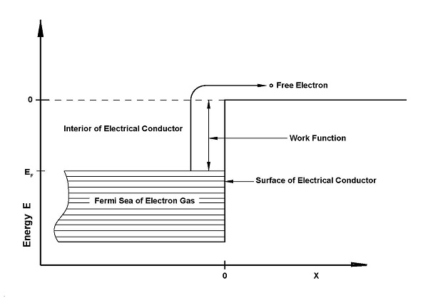
A Fermi Gas is a state of matter which is an ensemble of many non-interacting fermions. Fermions are particles that obey Fermi–Dirac statistics, like electrons, protons, and neutrons, and, in general, particles with half-integer spin. These statistics determine the energy distribution of fermions in a Fermi gas in thermal equilibrium, and is characterized by their number density, temperature, and the set of available energy states.
This physical model can be applied to the behaviour of charge carriers in a metal. The three-dimensional isotropic and non-relativistic uniform Fermi gas case is known as the Fermi sphere.
A three-dimensional infinite square well, (i.e. a cubical box that has a side length L) has the potential energy $ {\displaystyle V(x,y,z)= 0} $ for $ {\displaystyle - \frac {L}{2} \,\, < x,y,z < {\frac {L}{2}}} $
The states are now labelled by three quantum numbers $ {\displaystyle n_x} $ , $ {\displaystyle n_y} $ , and $ {\displaystyle n_z} $ . The single particle energies are:
$$ {\displaystyle E_{n_{x},n_{y},n_{z}}=E_{0}+{\frac {\hbar ^{2}\pi ^{2}}{2mL^{2}}}\left(n_{x}^{2}+n_{y}^{2}+n_{z}^{2}\right)\,,} $$Where $ {\displaystyle n_x} $ , $ {\displaystyle n_y} $ , $ {\displaystyle n_z} $ are positive integers.
To apply this model to our corona discharge model we must extend the model to the space where the box tends to the Thermodynamic limit. When the box contains $ {\displaystyle N} $ non-interacting fermions of spin $ {\displaystyle \frac {1}{2}} $ , we can calculate the energy in the thermodynamic limit, where $ {\displaystyle N} $ is so large that the quantum numbers $ {\displaystyle n_x} $ , $ {\displaystyle n_y} $ , $ {\displaystyle n_z} $ are treated as continuous variables.
With the vector $ {\displaystyle \mathbf {n} =(n_{x},n_{y},n_{z})} $ , each quantum state corresponds to a point in 'n-space' with energy:
$$ {\displaystyle E_{\mathbf {n} }=E_{0}+{\frac {\hbar ^{2}\pi ^{2}}{2mL^{2}}}|\mathbf {n} |^{2}\,} $$With $ {\displaystyle |\mathbf {n} |^{2}} $ denoting the square of the usual Euclidean length $ {\displaystyle |\mathbf {n} |={\sqrt {n_{x}^{2}+n_{y}^{2}+n_{z}^{2}}}} $ . The number of states with energy less than $ {\displaystyle E_F + E_0} $ is equal to the number of states that lie within a sphere of radius $ {\displaystyle |\mathbf {n} _{\mathrm {F} }|} $ in the region of n-space where $ {\displaystyle n_x} $ , $ {\displaystyle n_y} $ , $ {\displaystyle n_z} $ are positive. In the ground state this number equals the number of fermions in the system:
$$ {\displaystyle N=2\times {\frac {1}{8}}\times {\frac {4}{3}}\pi n_{\mathrm {F} }^{3}} $$The factor of two expresses the two spin states, and the factor of 1/8 expresses the fraction of the sphere that lies in the region where all $ {\displaystyle n} $ are positive.
$$ {\displaystyle n_{\mathrm {F} }=\left({\frac {3N}{\pi }}\right)^{1/3}} $$The Fermi energy is given by:
$$ {\displaystyle E_{\mathrm {F} }={\frac {\hbar ^{2}\pi ^{2}}{2mL^{2}}}n_{\mathrm {F} }^{2}={\frac {\hbar ^{2}\pi ^{2}}{2mL^{2}}}\left({\frac {3N}{\pi }}\right)^{2/3}} $$Which results in a relationship between the Fermi energy and the number of particles per volume:
: $$ {\displaystyle E_{\mathrm {F} }={\frac {\hbar ^{2}}{2m}}\left({\frac {3\pi ^{2}N}{V}}\right)^{2/3}} $$This is also the energy of the highest-energy particle (the $ {\displaystyle N^{th} } $ particle), above the zero point energy $ {\displaystyle E_{0}} $ . The $ {\displaystyle N'^{th}} $ th particle has an energy of:
$$ {\displaystyle E_{N'}=E_{0}+{\frac {\hbar ^{2}}{2m}}\left({\frac {3\pi ^{2}N'}{V}}\right)^{2/3}\,=E_{0}+E_{\mathrm {F} }{\big |}_{N'}} $$The total energy of a Fermi sphere of $ {\displaystyle N} $ fermions (which occupy all $ {\displaystyle N} $ energy states within the Fermi sphere) is given by:
$$ {\displaystyle E_{\rm {T}}=NE_{0}+\int _{0}^{N}E_{\mathrm {F} }{\big |}_{N'}\,dN'=\left({\frac {3}{5}}E_{\mathrm {F} }+E_{0}\right)N} $$Therefore, the average energy per particle is given by:
$$ {\displaystyle E_{\mathrm {av} }=E_{0}+{\frac {3}{5}}E_{\mathrm {F} }} $$Part 25.4: Field Emission Model
Electrons can be drawn out of a metal surface by high electrostatic fields. A high exterior static electric potential modifies the external potential barrier such that elctrons at or close to the fermi energy have a finite probability of tunneling through the potential barrier into the atmosphere.
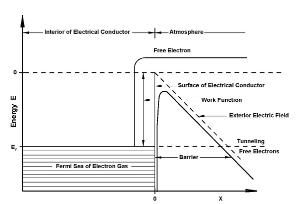
The following is a short introduction to the relevent Quantume Mechanical formulation required to understand the field emission theory of Fowler–Nordheim.
For an electron, inside a conducting metal, the one-dimensional Schrödinger equation can be written in the form:
$$ {\displaystyle {\frac {\hbar ^{2}}{2m}}{\frac {\mathrm {d} ^{2}\Psi (x)}{\mathrm {d} x^{2}}}=\left[U(x)-E_{\mathrm {n} }\right]\Psi (x)=M(x)\Psi (x),} $$where $ {\displaystyle \Psi (x)} $ is the electron wave-function, expressed as a function of distance $ {\displaystyle x} $ measured from the emitter's electrical surface, $ {\displaystyle \hbar} $ is the reduced Planck constant, $ {\displaystyle m} $ is the electron mass, $ {\displaystyle U(x)} $ is the electron potential energy, $ {\displaystyle E_n} $ is the total electron energy associated with motion in the x-direction, and $ {\displaystyle M(x) = [U(x) − E_n]} $ is called the electron motive energy. $ {\displaystyle M(x)} $ can be interpreted as the negative of the electron kinetic energy associated with the motion of a hypothetical classical point electron in the x-direction, and is positive in the barrier.
The shape of a tunneling barrier is determined by how $ {\displaystyle M(x)} $ varies with position in the region where $ {\displaystyle M(x) > 0} $ . Two models have special status in field emission theory: the exact triangular (ET) barrier and the Schottky–Nordheim (SN) barrier. These are given by the equations below:
$$ {\displaystyle M^{\mathrm {ET} }(x)=h-eFx} $$ $$ {\displaystyle M^{\rm {SN}}(x)=h-eFx-e^{2}/(16\pi \varepsilon _{0}x),} $$Here $ {\displaystyle h} $ is the zero-field height (or unreduced height) of the barrier, $ {\displaystyle e} $ is the elementary positive charge, $ {\displaystyle F} $ is the barrier field, and $ {\displaystyle \varepsilon _{0}} $ is the electric constant. By convention, $ {\displaystyle F} $ is taken as positive, even though the classical electrostatic field would be negative.
Escape probability: For an electron approaching the potential barrier from the inside, the probability of escape (or "transmission coefficient" is a function of $ {\displaystyle h} $ and $ {\displaystyle F} $ , and is denoted by $ {\displaystyle D(h,F)} $ . The primary problem of tunneling theory is to calculate $ {\displaystyle D(h,F)} $ . For physically realistic barrier models, such as the Schottky–Nordheim barrier, the Schrödinger equation cannot be solved exactly in any simple way. The following so-called "semi-classical" approach can be used. A parameter $ {\displaystyle G(h,F)} $ can be defined by the JWKB (Jeffreys-Wentzel-Kramers-Brillouin) integral:
$$ {\displaystyle G(h,F)=g\int M^{1/2}{\mbox{d}}x,} $$Where the integral is taken across the barrier, and the parameter $ {\displaystyle g} $ is a universal constant given by:
$$ {\displaystyle g\,=2{\sqrt {2m}}/\hbar \approx 10.24624\;{\rm {eV}}^{-1/2}\;{\rm {nm}}^{-1}.} $$Forbes has re-arranged a result proved by Fröman, to show that, in a one-dimensional treatment, the exact solution for $ {\displaystyle D} $ can be written:
$$ {\displaystyle \,D={\frac {P\mathrm {e} ^{-G}}{1+P\mathrm {e} ^{-G}}},} $$Where the tunneling pre-factor $ {\displaystyle P} $ can in principle be evaluated by complicated iterative integrations along a path in complex space. In the CFE regime we have (by definition) $ {\displaystyle G >> 1} $ . Also, for simple models $ {\displaystyle P = 1} $ . So the equation above reduces to the so-called simple JWKB formula:
$$ {\displaystyle D\approx P\mathrm {e} ^{-G}\approx \mathrm {e} ^{-G}.} $$For the exact triangular barrier, putting eq. (2) into eq. (4) yields $ {\displaystyle G^{ET} = bh^{3/2}/F} $ , where:
$$ {\displaystyle b={\frac {2g}{3e}}={\frac {4{\sqrt {2m}}}{3e\hbar }}\approx 6.830890\;{\mathrm {eV} }^{-3/2}\;\mathrm {V} \;{\mathrm {nm} }^{-1}.} $$This parameter $ {\displaystyle b} $ is a universal constant sometimes called the second Fowler–Nordheim constant. For barriers of other shapes, we write:
$$ {\displaystyle G(h,F)=\nu (h,F)G^{\mathrm {ET} }=\nu (h,F)bh^{3/2}/F,} $$Where $ {\displaystyle \nu (h,F)} $ is a correction factor that in general has to be determined by numerical integration.
Part 17.4: Fair Weather Electric Potential
Atmospheric electricity is always present, and during fine weather away from thunderstorms, the air above the surface of Earth is positively charged, while the Earth's surface charge is negative. This can be understood in terms of a difference of potential between a point of the Earth's surface, and a point somewhere in the air above it. Because the atmospheric electric field is negatively directed in fair weather, the convention is to refer to the potential gradient, which has the opposite sign and is about 100 V/m at the surface, away from thunderstorms.[4] There is a weak conduction current of atmospheric ions moving in the atmospheric electric field, about 2 picoamperes per square meter, and the air is weakly conductive due to the presence of these atmospheric ions.
Part 17.4.1: Fair Weather Electric Potential
The vertical atmospheric electric field, or Potential Gradient (PG), is a widely studied electrical property of the atmosphere. In fair weather and air unpolluted by aerosol particles, diurnal variations in PG result from changes in the total electrical output of global thunderstorms and shower clouds. Even early PG measurements, such as those obtained by Simpson (1906) in Lapland, show a variation suggestive of that seen in more modern work. A common global diurnal variation results from a diurnal variation in the ionospheric potential $ {\displaystyle V_1} $ , which modulates the vertical air-Earth conduction current $ {\displaystyle J_z} $ and, in the absence of local effects, the surface PG. $ {\displaystyle V_1} $ and $ {\displaystyle J_z} $ are parameters less prone to local microphysics effects and are therefore more suitable for the development of our model of negative-ion stimulation of precipitation.
Small ions are continually produced in the atmosphere by radiolysis of air molecules.
There are three major sources of high-energy particles, all of which cause ion production in air: radon isotopes, cosmic rays and terrestrial gamma radiation. The partitioning between the sources varies vertically. Near the surface over land, ionisation from turbulent transport of radon and other radioactive isotopes is important, together with gamma radiation from isotopes below the surface. Ionisation from cosmic rays is always present, comprising about 20% of the ionisation over the continental surface.
The cosmic ionisation fraction increases with increasing height in the atmosphere and dominates above the planetary boundary layer.
Part 17.4.2: Atmospheric Conductivity
After the PG, air conductivity is probably the second most frequently-measured surface quantity in atmospheric electricity. The slight electrical conductivity of atmospheric air results from the natural ionisation, generated by cosmic rays and background radioisotopes.
For bipolar ion number concentrations $ {\displaystyle n_+} $ and $ {\displaystyle n_-} $ the total air conductivity $ {\displaystyle \sigma} $ is given by:
$$ {\displaystyle \sigma = \sigma_+ + \sigma_- = e (\mu_+ n_+ + \mu_- n_ -)\,\,\,\,\,\,\,\,\,\,\,\,\,\,\,\,\,\,\,\,\,\,\,{\text{Equation 2.2.2.1}}}$$Part 17.4.3: Carnegie Diurnal Variations
The diurnal variation in PG identified in data obtained during the voyages of the Carnegie. As well as the surface PG, the universal diurnal or Carnegie curve appears in the other global circuit parameters, notably the ionospheric potential (Section 2.2.1) (Mülheisen, 1977) and air-Earth current.
A positive correlation between the Carnegie curve and diurnal variation in global thunderstorm area was discovered by Whipple, by summing the diurnal variations in thunderstorm area for each of Africa, Australia and America (Whipple, 1929; Whipple and Scrase, 1936). The thunderstorm areas were estimated using thunderday 4 statistics from meteorological stations, compiled by Brooks (1925).
Part 17.5: Electron Attachment and negative-ion creation
The work function of copper at 35 degrees Centigrade is approximately 4.7 Electron Volts. This implies that the corona electrons emmited from the negatively charged electrode have fairly high kinetic energy when they are released from the electrode into the ambient air. Coronas may be positive or negative. This is determined by the polarity of the voltage on the highly curved electrode. If the curved electrode is positive with respect to the flat electrode, it has a positive corona; if it is negative, it has a negative corona. The physics of positive and negative coronas are strikingly different. This asymmetry is a result of the great difference in mass between electrons and positively charged ions, with only the electron having the ability to undergo a significant degree of ionizing inelastic collision at common temperatures and pressures.
Part 17.6: Negatively charged aerosol Spray
There is a considerable variety in the sizes and abundance of aerosol particles, ice crystals and cloud droplets present in the atmosphere. The typical molecular cluster comprising an atmospheric small ion will have a diameter of less than one nanometre. Aerosols have diameters from 3nm to 10μm, and cloud and raindrops have diameters from 10μm to 1mm. The complexity of cloud microphysical processes results from both the different particle sizes and compositions in atmospheric clouds, and the phase changes between solid and liquid (Mason, 1971; Pruppacher and Klett, 1997).
Aerosol electrification in the atmosphere occurs from ion-aerosol attachment, facilitated by ion transport in electric fields (Pauthenier, 1956), by diffusion (Gunn 1955; Fuchs, 1963; Bricard, 1965; Boisdron and Brock, 1970).
Polar and chemical asymmetries in the ion properties generally result in a charge distribution on the aerosol, which, although the distribution may have a small mean charge, does not preclude the existence of transiently highly charged particles within the ensemble (Keep in mind that the charge density has the same distribution as the particle size but is not necessarily correlated to the size distribution. In the special case of negative-ion droplets created in the earth's boundary layer the charge arises from the ionization of air through a corona discharge mechanism which will be outlined elsewhere in this document. These ion will migrate to the upper part of the troposphere through the combined forces of difusion and the static electrical gradient in the planetary boundary layer.
Charge within the particle, and ions diffusing to the particle (Clement and Harrison, 1992; Gensdarmes et al., 2001). The aerosol charge distribution can affect aerosol coagulation rates (Clement et al., 1995), which in turn may modify the particle size distribution.
Section Eighteen: Negative-Ion Plume in PBL
Part 18.1: Aerosol Emission Plumes
Flow of aerosols in the form of negative-ions, charged water droplets, vapor or smoke released into the air at a very small altitude in surface layer of the planetary boundary layer. Plumes are of considerable importance in the atmospheric dispersion modelling of aerosols comenly refered to as air pollution. There are three primary types of aerosol emission plumes:
1. Buoyant Plumes
Plumes which are lighter than air because they are at a higher temperature and lower density than the ambient air which surrounds them, or because they are at about the same temperature as the ambient air but have a lower molecular weight and hence lower density than the ambient air. For example, the emissions from the flue gas stacks of industrial furnaces are buoyant because they are considerably warmer and less dense than the ambient air. As another example, an emission plume of methane gas at ambient air temperatures is buoyant because methane has a lower molecular weight than the ambient air.
2. Dense Gas Plumes
Plumes which are heavier than air because they have a higher density than the surrounding ambient air. A plume may have a higher density than air because it has a higher molecular weight than air (for example, a plume of carbon dioxide). A plume may also have a higher density than air if the plume is at a much lower temperature than the air. For example, a plume of evaporated gaseous methane from an accidental release of liquefied natural gas (LNG) may be as cold as -161 °C.
2. Passive or Neutral Plumes
Plumes which are neither lighter or heavier than air.
Part 18.1.1: Aerosol Dispersion Models
We will only discuss two of the five most often quoted types of aerosol dispersion models:
1. Box Model: The box model is the simplest of the model types. It assumes the air control volume (i.e., a given volume of atmospheric air in a geographical region) is in the shape of a box. It also assumes that the aerosols inside the box are homogeneously distributed and uses that assumption to estimate the average aerosol concentrations anywhere within the control volume. Although useful, this model is very limited in its ability to accurately predict dispersion of aerosols over the base of the control volume area because the assumption of a homogeneous distribution of aerosols into the lower stratum of the boundary layer is much too simple.
2. Gaussian model: The Gaussian model is the oldest and the most commonly used model type. It assumes that the aerosol dispersion has a Gaussian distribution. This means that the aerosol distribution has a normal probability distribution. Gaussian models are most often used for predicting the dispersion of continuous, buoyant aerosol plumes originating from ground-level or elevated sources. We will be discussing this model at lenght since it is appropriate for the physics which we are developing for the dispersion of negative-ion aerosols and negatively charged aerosol sprays at less than thirty feet of altitude above the planetary surface in our control volume area which we will refer to as our Source Footprint.
The primary computational algorithm used in Gaussian modeling is the Generalized Dispersion Equation For A Continuous Point-Source Plume. $$ {\displaystyle C={\frac {\;Q}{u}}\cdot {\frac {\;f}{\sigma _{y}{\sqrt {2\pi }}}}\;\cdot {\frac {\;g_{1}+g_{2}+g_{3}}{\sigma _{z}{\sqrt {2\pi }}}}} $$
Where:
$ {\displaystyle f} $ = crosswind dispersion parameter:
$ {\displaystyle f = \exp (-y^{2} /(2 \sigma _{y}^{2}))} $
$ {\displaystyle g}$ = vertical dispersion parameter = $ {\displaystyle g_1 + g_2} $
$ {\displaystyle g_{1}} $ vertical dispersion with no reflections = $ {\displaystyle \exp (-(z-H)^{2}/(2 \sigma _{z}^{2}\;)\;]} $
$ {\displaystyle g_{2}} $ vertical dispersion for reflection from the ground = $ {\displaystyle \exp (-(z+H)^{2}/\,(2\;\sigma _{z}^{2}))} $
$ {\displaystyle C} $ concentration of emissions, in $ {\displaystyle g / m^3} $ , at any receptor located:
$ {\displaystyle x} $ meters downwind from the emission source point
$ {\displaystyle y} $ meters crosswind from the emission plume centerline
$ {\displaystyle z} $ meters above ground level
$ {\displaystyle Q} $ Q is the source aerosol emission rate,
$ {\displaystyle u} $ u is the horizontal wind velocity along the plume centerline,
$ {\displaystyle H} $ H is the height of emission plume centerline above ground level,
$ {\displaystyle \sigma_z} $ σ is the vertical standard deviation of the emission distribution,
$ {\displaystyle \sigma_y} $ σ is the horizontal standard deviation of the emission distribution,
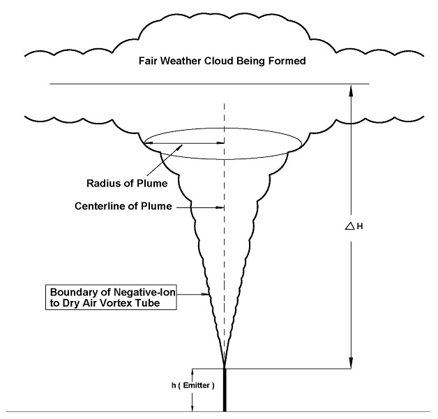
$ {\displaystyle \sigma_z} $ and $ {\displaystyle \sigma_y} $ are functions of the atmospheric stability class (i.e., a measure of the turbulence in the ambient atmosphere) and of the downwind distance to the receptor. The two most important variables affecting the degree of aerosol emission dispersion obtained are the height of the emission source point and the degree of atmospheric turbulence.
Plume rise is a very important factor in determining maximum ground-level concentrations from most sources since it typically increases the effective stack height by a factor of 2 to 10 times the actual release height. Because maximum ground-level concentration is roughly proportional to the inverse square of the effective stack height, it is clear that plume rise can reduce ground-level concentration by a factor of as much as 100. Most industrial pollutants are emitted with high velocity or temperature, and plume rise must be calculated. However, pollutants released from some building vents or motor vehicles have very little plume rise.
A few areas of plume rise are well understood, such as the trajectory before final rise is reached and final rise in stable conditions. In both of these cases, the effect of ambient turbulence in the air outside the plume is negligible. When ambient turbulence affects the plume, such as during final rise in neutral conditions and during the last half of rise in convective conditions, the models are less certain, and more research is needed.
The review article by Brigs (1975) provides background material on available plume-rise models. Most models are based on fundamental laws of fluid mechanics: conservation of mass, potential density, and momentum. The distribution of temperature, speed, or other quantities across the plume is assumed to have “ top hat ” form; that is, a variable has a certain value inside the plume, another value outside the plume, and a discontinuity at the plume radius (R). Basically we are looking at integrated averages of variables in a plume cross section. The figure below is a schematic drawing of a vertical plume model which we are using and which illustrates many of the variables and parameters important in calculating plume rise. A plume is usually more or less “vertical” if wind speed is less than about 1 m/sec.
Note the difference on the figure in definitions of the plume volume flux :
The Gaussian air pollutant dispersion equation (discussed above) requires the input of H which is the pollutant plume's centerline height above ground level—and H is the sum of Hs (the actual physical height of the pollutant plume's emission source point) plus ΔH (the plume rise due to the plume's buoyancy).
To determine ΔH, many if not most of the air dispersion models developed between the late 1960s and the early 2000s used what are known as "the Briggs equations." G.A. Briggs first published his plume rise observations and comparisons in 1965.[9] In 1968, at a symposium sponsored by CONCAWE (a Dutch organization), he compared many of the plume rise models then available in the literature.[10] In that same year, Briggs also wrote the section of the publication edited by Slade[11] dealing with the comparative analyses of plume rise models. That was followed in 1969 by his classical critical review of the entire plume rise literature, in which he proposed a set of plume rise equations which have become widely known as "the Briggs equations". Subsequently, Briggs modified his 1969 plume rise equations in 1971 and in 1972.