CHAPTER ZERO

1.    This webpage is being developed by the Senior Engineer of AscenTrust, LLc.

2.   The Senior Engineer is a Graduate of Electrical and Computing Engineering (University of Alberta, Edmonton) and Graduated with Distinction in 1969

3.    This document is meant as an introduction to the broad subject of Human Physiological Systems. The organ analysis of the human body has failed miserably maily due to its lack of inclusion of the interconnection of primary physiological systems to each and every organ system. We will be concentrating our efforts, in this document on the two most important controlling systems in the human body. These are the nervous system and the Cardio-vascular system. The final aim of this document will be to analyse the interaction of the nervous system with the neurons that control the sinoatrial node in order to gain some understanding of what causes Atrial Fibrilation.

4.   This webpage is in a state of ongoing development and new material will appear from time to time as the workload permits.

5.    The text and mathematical equations below are renderred in HTML using a web-based Latex and Javascript renderring engine.

PROLEGOMENA

We Human Beings are often characterized as an evolutionary improvement of an ape-like antecedent. This notion was systematized by Darwin and gained general scientific acceptance after he published On the Origin of Species in 1859. This assumption should have died in 1957 when Watson and Crick laid out the central dogma of molecular biology, which foretold the relationship between DNA, RNA, and proteins, and articulated the "adaptor hypothesis".

Final confirmation of the replication mechanism that was implied by the double-helical structure followed in 1958 through the Meselson–Stahl experiment. Further work by Crick and co-workers showed that the genetic code was based on non-overlapping triplets of bases, called codons, allowing Har Gobind Khorana, Robert W. Holley, and Marshall Warren Nirenberg to decipher the genetic code.

The majority of modern research in human physiolgy is concerned with the creation of fairly simple, graphical, linear models. These models are not meant to simulate human physiologicl processes.

Section one: Worldview

Before we begin our analysis of human physiolgy systems we need to address the philosophical presupositions of our theses and how it differs from the commonly held belief in rationalism and materialism. The notions of Physics, Metaphysics, Ontology, Epistomology and Worldview

Artificial Intelligence Academics involved in the computing Science and Engineering of systems have variously proposed definitions of intelligence that include the intelligence demonstrated by machines. Some of these definitions are meant to be general enough to encompass human intelligence as well. An intelligent agent can be defined as a system that perceives its environment and takes actions which maximize its chances of success. It is clear that these systems cannot be modelled only in software.

Kaplan and Haenlein define artificial intelligence as "a system's ability to correctly interpret external data, to learn from such data, and to use those learnings to achieve specific goals and tasks through flexible adaptation". Progress in artificial intelligence has been limited to very narrow ranges of mainly software computational modeling which includes machine learning, deep learning and deep neural networks. All existing AI systems lack the most fundamental part of what makes a human being different from all other entities in the Creation, that being the Spirit

Atheistic Materialism is a form of philosophical monism in metaphysics, according to which matter is the fundamental substance in nature, and all things, including mental states and consciousness, are results of material interactions. According to philosophical materialism, mind and consciousness are caused by physical processes, such as the neurochemistry of the human brain and nervous system, without which they cannot exist. Materialism directly contrasts with monistic idealism, according to which consciousness is the fundamental substance of nature.

Dualism:The term dualism, in this document, is employed in opposition to the Atheistic presuposition of monism (The Cosmos consists of only one substance), to signify the ordinary view that the existing universe contains two radically distinct kinds of being or substance — matter and spirit, body and mind. Dualism is thus opposed to both materialism and idealism. Idealism, however, of the Berkeleyan type, which maintains the existence of a multitude of distinct substantial minds, may along with dualism, be described as pluralism. philosophical view which holds that mental phenomena are, at least in certain respects, not physical phenomena, or that the mind and the body are distinct and separable from one another.

Epistomology:: In this document we shall consider epistemology in its historical and broader meaning, which is the usual one in English, as applying to the theory of knowledge. Epistomology is therefore understood as that part of Philosophy which describes, analyses and examines the facts of knowledge as such and then tests chiefly the value of knowledge and of its various kinds, its conditions of validity, range and limits (critique of knowledge).

Intelligence: Human intelligence is marked by complex cognitive feats and high levels of motivation and self-awareness. Intelligence enables humans to remember descriptions of things and use those descriptions in future behaviors. It is a cognitive process. It gives humans the cognitive abilities to learn, form concepts, understand, and reason, including the capacities to recognize patterns, innovate, plan, solve problems, and employ language to communicate. Intelligence enables humans to experience and think.

Intelligence is different from learning. Learning refers to the act of retaining facts and information or abilities and being able to recall them for future use, while intelligence is the cognitive ability of someone to perform these and other processes. There are various tests which accurately quantify intelligence, such as the Intelligence Quotient (IQ) test.

Mind::The mind is that which thinks, feels, perceives, imagines, remembers, and wills. It covers the totality of mental phenomena, including both conscious processes, through which an individual is aware of external and internal circumstances, and unconscious processes, which can influence an individual without intention or awareness. The mind plays a central role in most aspects of human life, but its exact nature is disputed. Some characterizations focus on internal aspects, saying that the mind transforms information and is not directly accessible to outside observers. Others stress its relation to outward conduct, understanding mental phenomena as dispositions to engage in observable behavior.The mind–body problem is the challenge of explaining the relation between matter and mind. Traditionally, mind and matter were often thought of as distinct substances that could exist independently from one another. The dominant philosophical position since the 20th century has been physicalism, which says that everything is material, meaning that minds are certain aspects or features of some material objects.

Monism::The monist holds that the whole is prior to its parts, and thus views the cosmos as fundamental, with metaphysical explanation dangling downward from the One. The pluralist holds that the parts are prior to their whole, and thus tends to consider particles fundamental, with metaphysical explanation snaking upward from the many. Just as the materialist and idealist debate which properties are fundamental, so the monist and pluralist debate which objects are fundamental. I will defend the monistic view. In particular I will argue that there are physical and modal considerations that favor the priority of the whole.Physically, there is good evidence that the cosmos forms an entangled system and good reason to treat entangled systems as irreducible wholes.Modally,mereology allows for the possibility of atomlessgunk , with no ultimate parts for the pluralist to invoke as the ground of being.

Ontology: Though the use of the term has its roots in the Greek Physics and Metaphysics its modern use goes back to Clauberg (1625-1665), its special application to the first discussions of metaphysical concepts was made by Christian von Wolff (1679-1754). Prior to this time "the science of being" had retained the titles given it by its founder Aristotle: "first philosophy", "theology", "wisdom". The term "metaphysics" was given a wider extension by Wolff, who divided "real philosophy" into general metaphysics, which he called ontology, and special, under which he included cosmology, psychology, and theodicy.

Worldview: One's worldview comprises a number of basic beliefs which provide the philosophical and ethical underpinning of an individuals behavioral patterns. These basic beliefs cannot, by definition, be proven (in the logical sense) within the worldview – precisely because they are axioms, and are typically argued from rather than argued for.

If two different worldviews have sufficient common beliefs it may be possible to have a constructive dialogue between them.

On the other hand, if different worldviews are held to be basically incommensurate and irreconcilable, then the situation is one of cultural relativism and would therefore incur the standard criticisms from philosophical realists. Additionally, religious believers might not wish to see their beliefs relativized into something that is only "true for them". Subjective logic is a belief-reasoning formalism where beliefs explicitly are subjectively held by individuals but where a consensus between different worldviews can be achieved.

Section Two: Models and Reality

The Academic idea that modelling and simulations can bring us to an understanding of reality is most certainly false. Certainly, modelling has become an essential and inseparable part of many scientific disciplines, each of which has its own ideas about specific types of modelling. The following was said by John von Neumann:

... the sciences do not try to explain, they hardly even try to interpret, they mainly make models. By a model is meant a mathematical construct which, with the addition of certain verbal interpretations, describes observed phenomena. The justification of such a mathematical construct is solely and precisely that it is expected to work—that is, correctly to describe phenomena from a reasonably wide area.

A model seeks to represent empirical objects, phenomena, and physical processes in a logical and objective way. All models are in simulacra, that is, simplified reflections of reality that, despite being approximations, can be extremely useful. Building and disputing models is fundamental to the Academic enterprise. Complete and true representation are impossible, but Academics debate often concerns which is the better model for a given task, e.g., which is the more accurate climate model for seasonal forecasting.

Attempts to formalize the principles of the empirical sciences use an interpretation to model reality, in the same way logicians axiomatize the principles of logic. The aim of these attempts is to construct a formal system that will not produce theoretical consequences that are contrary to what is found in reality. Predictions or other statements drawn from such a formal system mirror or map the real world only insofar as these scientific models are true.

For the researcher, a model is also a way in which the human thought processes can be amplified. For instance, models that are rendered in software allow programmmers to leverage computational power to simulate, visualize and manipulate the entity, phenomenon, or process being represented.

Section Three:   Prototypes

A prototype is an early physical model of a product built to test a concept or process. It is a term used in a variety of contexts, including semantics, design, electronics, and software programming. A prototype is generally used to evaluate a new design to enhance precision by system analysts and users and in our case to do value Engineering on the Product. Prototyping serves to provide specifications for a real, working system rather than a theoretical one. In some design workflow models, creating a prototype (a process sometimes called materialization) is the step between the formalization and the evaluation of an idea.

Prototypes explore the different aspects of an intended design:

1.   A proof-of-principle prototype serves to verify some key functional aspects of the intended design, but usually does not have all the functionality of the final product.

2.   A working prototype represents all or nearly all of the functionality of the final product.

3.   A visual prototype represents the size and appearance, but not the functionality, of the intended design. A form study prototype is a preliminary type of visual prototype in which the geometric features of a design are emphasized, with less concern for color, texture, or other aspects of the final appearance.

4.   A user experience prototype represents enough of the appearance and function of the product that it can be used for user research.

5.   A functional prototype captures both function and appearance of the intended design, though it may be created with different techniques and even different scale from final design.

6.   A paper prototype is a printed or hand-drawn representation of the user interface of a software product. Such prototypes are commonly used for early testing of a software design, and can be part of a software walkthrough to confirm design decisions before more costly levels of design effort are expended.

Section Four:   Value Engineering

Value Engineering is a systematic analysis of the various components and materials of a system (The system under discussion in this document is the cardio-vascular system of the human body) in order to improve the performance or functionality of the sysstem. In the case of the onset of atrial fibrilation in the cardio-vascular system, the first round of Value Engineering will consist of analysis of the neural interconnect to the sinoatrial node of the heart. The sinoatrial node is responsible for the initiation of the neural pulses which control the beating of the heart.

Value engineering is a key part of all Research and Development Projects within the biomedical engineering, industrial engineering or architecture body of knowledge as a technique in which the value of a system’s outputs is superficially optimized by distorting a mix of performance (function) and costs. It is based on an analysis investigating systems, equipment, facilities, services, and supplies for providing necessary functions at superficial low life cycle cost while meeting the misunderstood requirement targets in performance, reliability, quality, and safety. In most cases this practice identifies and removes necessary functions of value expenditures, thereby decreasing the capabilities of the manufacturer and/or their customers. What this practice disregards in providing necessary functions of value are expenditures such as equipment maintenance and relationships between employee, equipment, and materials. For example, a machinist is unable to complete their quota because the drill press is temporarily inoperable due to lack of maintenance and the material handler is not doing their daily checklist, tally, log, invoice, and accounting of maintenance and materials each machinist needs to maintain the required productivity and adherence to section 4306.

VE follows a structured thought process that is based exclusively on "function", i.e. what something "does", not what it "is". For example, a screwdriver that is being used to stir a can of paint has a "function" of mixing the contents of a paint can and not the original connotation of securing a screw into a screw-hole. In value engineering "functions" are always described in a two word abridgment consisting of an active verb and measurable noun (what is being done – the verb – and what it is being done to – the noun) and to do so in the most non-descriptive way possible. In the screwdriver and can of paint example, the most basic function would be "blend liquid" which is less descriptive than "stir paint" which can be seen to limit the action (by stirring) and to limit the application (only considers paint).

Value engineering uses rational logic (a unique "how" - "why" questioning technique) and an irrational analysis of function to identify relationships that increase value. It is considered a quantitative method similar to the scientific method, which focuses on hypothesis-conclusion approaches to test relationships, and operations research, which uses model building to identify predictive relationships.

Section Five:   Physiological Systems

Human physiology is the study of how the human body's systems and functions work together to maintain a stable internal environment. It includes the study of the nervous, endocrine, cardiovascular, respiratory, digestive, and urinary systems, as well as cellular and exercise physiology. Understanding human physiology is essential for diagnosing and treating health conditions and promoting overall wellbeing.

It seeks to understand the systems that work together to keep the human body alive and functioning. The principal level of focus of physiology is at the level of organs and systems within systems. The nervous systems and the endocrine systems play major roles in the reception and transmission of signals that integrate function in human systems. Homeostasis is a major aspect with regard to such interactions within the circulatory systems of humans. The biological basis of the study of physiology, integration refers to the overlap of many functions of the systems of the human body, as well as its accompanied form. It is achieved through communication that occurs in a variety of ways, both electrical and chemical.

The following is a list of the main physiological systems in the human body. A physiological system is a group of organs that work together to perform major functions or meet physiological needs of the body.

1.    Cardiovascular system: Transportation of oxygen, nutrients and hormones throughout the body and elimination of cellular metabolic waste.

2.    Central Nervous system: Initiation and regulation of vital body functions, sensation and body movements. The central nervous sytem is the feedback and control system that controls all of the interactions of the internal systems with the external environment.

3.    Musculoskeletal system: Mechanical support, posture and locomotion.

4.    Respiratory system: Exchange of oxygen and carbon-dioxide between the body and air, acid-base balance regulation, phonation.

5.    Digestive system: Mechanical and chemical degradation of food with purpose of absorbing into the body and using as energy.

6.    Urinary system: Filtration of blood and eliminating unnecessary compounds and waste by producing and excreting urine.

7.   Endocrine system: Production of hormones in order to regulate a wide variety of bodily functions (e.g. menstrual cycle, sugar levels, etc)

8.    Lymphatic system: Draining of excess tissue fluid, immune defense of the body.

9.   Reproductive system: Production of reproductive cells and contribution towards the reproduction process.

10.   Integumentary system: Physical protection of the body surface, sensory reception, vitamin synthesis.

Chapter One:   The cardio-vascular system

In humans, the circulatory system is a system of organs that includes the heart, blood vessels, and blood which is circulated throughout the body. It includes the cardiovascular system, or vascular system, that consists of the heart and blood vessels (from Greek kardia meaning heart, and Latin vascula meaning vessels). The circulatory system has two divisions, a systemic circulation or circuit, and a pulmonary circulation or circuit. Some sources use the terms cardiovascular system and vascular system interchangeably with circulatory system.

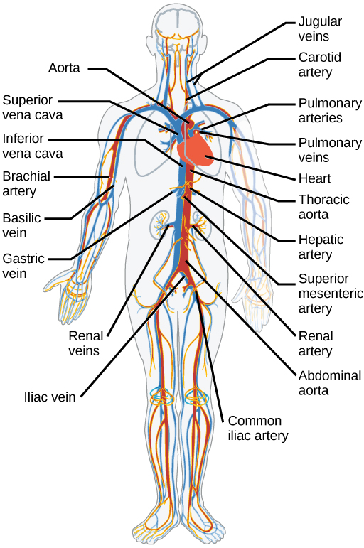
The network of blood vessels are the great vessels of the heart including large elastic arteries, and large veins; other arteries, smaller arterioles, capillaries that join with venules (small veins), and other veins. The circulatory system of humans is closed, which means that the blood never leaves the network of blood vessels.

Blood is a fluid consisting of plasma, red blood cells, white blood cells, and platelets; it is circulated around the body carrying oxygen and nutrients to the tissues and collecting and disposing of waste materials. Circulated nutrients include proteins and minerals and other components include hemoglobin, hormones, and gases such as oxygen and carbon dioxide. These substances provide nourishment, help the immune system to fight diseases, and help maintain homeostasis by stabilizing temperature and natural pH.

The circulatory system can be affected by many cardiovascular diseases. Cardiologists are medical professionals which specialise in the heart, and cardiothoracic surgeons specialise in operating on the heart and its surrounding areas. Vascular surgeons focus on disorders of the blood vessels, and lymphatic vessels.

Chapter Two:   The Nervous System

The human nervous system is a highly complex and interconnected system that coordinates our actions and sensory information by transmitting signals to and from different parts of its body. The nervous system detects environmental changes that impact the body, then works in tandem with the endocrine system to respond to such events.

The nervous systems consists of two main parts, the central nervous system (CNS) and the peripheral nervous system (PNS).

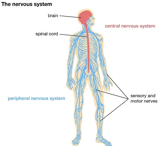
The central nervous system (CNS) consists of the brain and spinal cord. The peripheral nervous system (PNS) consists mainly of nerves, which are enclosed bundles of the long fibers, or axons, that connect the CNS to every other part of the body.

Nerves that transmit signals from the brain are called motor nerves (efferent), while those nerves that transmit information from the body to the CNS are called sensory nerves (afferent).

The peripheral nervous system (PNS) is divided into two separate subsystems, the somatic and autonomic nervous systems. The autonomic nervous system is further subdivided into the sympathetic, parasympathetic and enteric nervous systems. The sympathetic nervous system is activated in cases of emergencies to mobilize energy, while the parasympathetic nervous system is activated when the body is in a relaxed state. The enteric nervous system functions to control the gastrointestinal system.

Nerves that exit from the brain are called cranial nerves while those exiting from the spinal cord are called spinal nerves.

Chapter Three:   Musculoskeletal system

The human musculoskeletal system is a physiological system that gives humans the ability to move using their muscular and skeletal systems. The musculoskeletal system provides form, support, stability, and movement to the body.

The human musculoskeletal system is made up of the bones of the skeleton, muscles, cartilage, tendons, ligaments, joints, and other connective tissue that supports and binds tissues and organs together. The musculoskeletal system's primary functions include supporting the body, allowing motion, and protecting vital organs.

This system describes how bones are connected to other bones and muscle fibers via connective tissue such as tendons and ligaments. The bones provide stability to the body. Muscles keep bones in place and also play a role in the movement of bones. To allow motion, different bones are connected by joints. Cartilage prevents the bone ends from rubbing directly onto each other.

Muscles contract to move the bone attached at the joint.

There are three types of muscles—cardiac, skeletal, and smooth.

1.    Cardiac Muscles: Skeletal and cardiac muscles have striations that are visible under a microscope due to the components within their cells. Cardiac muscles are very special muscles and found only in the heart and are used only to circulate blood; like the smooth muscles, these muscles are not under conscious control. Muscles are innervated, whereby nervous signals are communicated by nerves, which conduct electrical currents from the central nervous system and cause the muscles to contract.

2.    Skeletal Muscles: Only skeletal and smooth muscles are part of the musculoskeletal system and only the muscles can move the body.Skeletal muscles are attached to bones and arranged in opposing groups around joints. Muscles are innervated, whereby nervous signals are communicated[9] by nerves, which conduct electrical currents from the central nervous system and cause the muscles to contract.

3.    Smooth Muscles: Smooth muscles are used to control the flow of substances within the lumens of hollow organs, and are not consciously controlled. Skeletal and cardiac muscles have striations that are visible under a microscope due to the components within their cells. Only skeletal and smooth muscles are part of the musculoskeletal system and only the muscles can move the body. Cardiac muscles are found in the heart and are used only to circulate blood; like the smooth muscles, these muscles are not under conscious control. Skeletal muscles are attached to bones and arranged in opposing groups around joints.[8] Muscles are innervated, whereby nervous signals are communicated by nerves, which conduct electrical currents from the central nervous system and cause the muscles to contract.

There are, however, diseases and disorders that may adversely affect the function and overall effectiveness of the system. These diseases can be difficult to diagnose due to the close relation of the musculoskeletal system to other internal systems. The musculoskeletal system refers to the system having its muscles attached to an internal skeletal system and is necessary for humans to move to a more favorable position. Complex issues and injuries involving the musculoskeletal system are usually handled by a physiatrist (specialist in physical medicine and rehabilitation) or an orthopaedic surgeon.

Chapter Four:   The Normal heart

The heart is the muscular organ at the center of the cardio-vascular system. This organ pumps blood through the blood vessels. The heart and blood vessels together make the cardio-vascular or circulatory system. The pumped blood carries oxygen and nutrients to the tissue, while carrying metabolic waste such as carbon dioxide to the lungs. In humans, the heart is approximately the size of a closed fist and is located between the lungs, in the middle compartment of the chest, called the mediastinum.

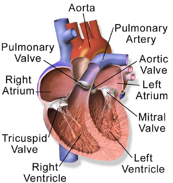
The normal human heart is divided into four chambers: upper left and right atria and lower left and right ventricles. Commonly, the right atrium and ventricle are referred together as the right heart and their left counterparts as the left heart. In a healthy heart, blood flows one way through the heart due to heart valves, which prevent backflow.

The heart is enclosed in a protective sac, the pericardium, which also contains a small amount of fluid. The wall of the heart is made up of three layers: epicardium, myocardium, and endocardium.

The normal heart pumps blood with a rhythm determined by a group of pacemaker cells in the sinoatrial node. These generate an electric current that causes the heart to contract, traveling through the atrioventricular node and along the conduction system of the heart.

In humans, deoxygenated blood enters the heart through the right atrium from the superior and inferior venae cavae and passes to the right ventricle. From here, it is pumped into pulmonary circulation to the lungs, where it receives oxygen and gives off carbon dioxide. Oxygenated blood then returns to the left atrium, passes through the left ventricle and is pumped out through the aorta into systemic circulation, traveling through arteries, arterioles, and capillaries—where nutrients and other substances are exchanged between blood vessels and cells, losing oxygen and gaining carbon dioxide—before being returned to the heart through venules and veins. The adult heart beats at a resting rate close to 72 beats per minute.

Chapter Five:   Cardiac Rhythms

The normal heart pumps blood with a rhythm determined by a group of pacemaker cells in the sinoatrial node. These generate an electric current that causes the heart to contract, traveling through the atrioventricular node and along the conduction system of the heart.

Section one: Introduction

APPENDIX ONE:   MATHEMATICAL PRELIMINARIES

This chapter of this webpage will provide the reader with an absolute minimum of the mathematical background required for even a small understanding of a small part of basic mathematical structures required for a basic understanding of Newtonian Mechanical Theory, the Mechanical theories of Hamilton and Lagrange, the Electromagnetic Theory of Maxwell's, electrical circuit theory of Kirchoff and the Quantum Theory of Schrödinger. We will be using the Harmonic Oscillator Model as a minimum requirement for the study of Power Systems and Nuclear Reactor Theory. We therefore adopt a practical view (Engineering) of Model Building. This implies: All models are a lie but some models are useful!. We will be comparing the analysis of the harmonic oscillator in many representations.

Section One:   Sets and Functions

Part One: Sets

A set is the mathematical model for a collection of different objects or things; a set contains elements or members, which can be mathematical objects of any kind: numbers, symbols, points in space, lines, other geometrical shapes, variables, or even other sets. The set with no element is the empty set; a set with a single element is a singleton. A set may have a finite number of elements or be an infinite set. Two sets are equal if they have precisely the same elements. Sets form the basis in modern mathematics and provide a common starting point for many areas of science and Engineering. The use of Boolean Logic in the layout of Computer chips is strongly influenced by the theories of Sets.

Set-builder notation can be used to describe a set that is defined by a predicate, that is, a logical formula that evaluates to true for an element of the set, and false otherwise. In this form, set-builder notation has three parts: a variable, a colon or vertical bar separator, and a predicate. Thus there is a variable on the left of the separator, and a rule on the right of it. These three parts are contained in curly brackets: $$ {\displaystyle \{x\mid \Phi (x)\}} $$ or $$ {\displaystyle \{x:\Phi (x)\}.} $$

The vertical bar (or colon) is a separator that can be read as "such that", "for which", or "with the property that". The formula $ {\displaystyle \Phi (x)} $ is said to be the rule or the predicate. All values of $ {\displaystyle x} $ for which the predicate holds (is true) belong to the set being defined. All values of $ {\displaystyle x} $ for which the predicate does not hold do not belong to the set. Thus $ {\displaystyle \{x\mid \Phi (x)\}} $ is the set of all values of $ {\displaystyle x} $ that satisfy the formula $ {\displaystyle \Phi} $ . It may be the empty set, if no value of $ {\displaystyle x} $ satisfies the formula.

Part Two: Introduction to Functions

A function from a set X to a set Y is an assignment of an element of Y to each element of X. The set X is called the domain of the function and the setY is called the codomain or range of the function.

A function, its domain, and its codomain, are declared by the notation f: X→Y, and the value of a function f at an element x of X, denoted by f(x), is called the image of x under f, or the value of f applied to the argument x. Functions are also called maps or mappings.

Two functions f and g are equal if their domain and codomain sets are the same and their output values agree on the whole domain. More formally, given f: X → Y and g: X → Y, we have f = g if and only if f(x) = g(x) for all x ∈ X. The range or image of a function is the set of the images of all elements in the domain.

Part Three: Important Functions

1.   Trigonometric Functions:

Trigonometric functions (also called circular functions) are real functions which relate an angle of a right-angled triangle to ratios of two side lengths. They are widely used in Engineering and form the basis for the analysis of circulation models of the atmosphere. They are the simplest periodic functions, and as such are widely used in the study of elctrodynamic phenomena through Fourier analysis.

The trigonometric functions most widely used in modern mathematics are the sine, the cosine, and the tangent. Their reciprocals are respectively the cosecant, the secant, and the cotangent, which are less used. Each of these six trigonometric functions has a corresponding inverse function, and an analog among the hyperbolic functions.

The oldest definitions of trigonometric functions, related to right-angle triangles, define them only for acute angles. To extend the sine and cosine functions to functions whose domain is the whole real line, geometrical definitions using the standard unit circle (i.e., a circle with radius 1 unit) are often used; then the domain of the other functions is the real line with some isolated points removed. Modern definitions express trigonometric functions as infinite series or as solutions of differential equations. This allows extending the domain of sine and cosine functions to the whole complex plane, and the domain of the other trigonometric functions to the complex plane with some isolated points removed.

$$ {\displaystyle \sin \theta ={\frac {\mathrm {opposite} }{\mathrm {hypotenuse} }}}\,\,\,\,\,\,\,\,\,\,\,\,\,\,\,\,\,\,\,\,\,\,\, {\displaystyle \csc \theta ={\frac {\mathrm {hypotenuse} }{\mathrm {opposite} }}}$$ $$ {\displaystyle \cos \theta ={\frac {\mathrm {adjacent} }{\mathrm {hypotenuse} }}} \,\,\,\,\,\,\,\,\,\,\,\,\,\,\,\,\,\,\,\,\,\,\, {\displaystyle \sec \theta ={\frac {\mathrm {hypotenuse} }{\mathrm {adjacent} }}}$$ $$ {\displaystyle \tan \theta ={\frac {\mathrm {opposite} }{\mathrm {adjacent} }}}\,\,\,\,\,\,\,\,\,\,\,\,\,\,\,\,\,\,\,\,\,\,\, {\displaystyle \cot \theta ={\frac {\mathrm {adjacent} }{\mathrm {opposite} }}}$$

  

2.   The Logarithmic Function:

In mathematics, the logarithm is the inverse function to exponentiation. That means the logarithm of a given number x is the exponent to which another fixed number, the base b, must be raised, to produce that number x. In the simplest case, the logarithm counts the number of occurrences of the same factor in repeated multiplication; e.g. since $ {\displaystyle {1000 = 10 × 10 × 10 = 10^3}}$ , the "logarithm base 10" of 1000 is 3, or log10 (1000) = 3. The logarithm of x to base b is denoted as $ log_b (x)$ .

The logarithm base 10 (that is b = 10) is called the decimal or common logarithm and is commonly used in engineering and Computer Science. The natural logarithm has the number e (that is b ≈ 2.718) as its base; its use is widespread in Engineering, mathematics and physics, because of its simpler integral and derivative. The binary logarithm uses base 2 (that is b = 2) and is frequently used in computer science.

Logarithms were introduced by John Napier in 1614 as a means of simplifying calculations. They were rapidly adopted by navigators, scientists, engineers, surveyors and others to perform high-accuracy computations more easily. Using logarithm tables, tedious multi-digit multiplication steps can be replaced by table look-ups and simpler addition. This is possible because of the fact that the logarithm of a product is the sum of the logarithms of the factors: $$ {\displaystyle \log _{b}(xy)=\log _{b}x+\log _{b}y.}$$ provided that b, x and y are all positive and b ≠ 1. The slide rule, also based on logarithms, allows quick calculations without tables, but at lower precision. The present-day notion of logarithms comes from Leonhard Euler, who connected them to the exponential function in the 18th century, and who also introduced the letter e as the base of natural logarithms.

Logarithmic scales reduce wide-ranging quantities to smaller scopes. For example, the decibel (dB) is a unit used to express ratio as logarithms, mostly for signal power and amplitude (of which sound pressure is a common example). Logarithms are commonplace in Engineeering and in measurements of the complexity of algorithms.

3.   The Exponential Function:

The exponential function is a mathematical function denoted by $ {\displaystyle f(x)=\exp(x)}$ or $ {\displaystyle e^{x}}$ (where the argument x is written as an exponent). Unless otherwise specified, the term generally refers to the positive-valued function of a real variable, although it can be extended to the complex numbers or generalized to other mathematical objects like matrices or Lie algebras. The exponential function originated from the notion of exponentiation (repeated multiplication), but modern definitions (there are several equivalent characterizations) allow it to be rigorously extended to all real arguments, including irrational numbers. Its application in Engineering qualifies the exponential function as one of the most important function in mathematics.

The exponential function satisfies the exponentiation identity: $ {\displaystyle e^{x+y}=e^{x}e^{y}{\text{ for all }}x,y\in \mathbb {R} ,}$ which, along with the definition $ {\displaystyle e=\exp(1)}$ , shows that $ {\displaystyle e^{n}=\underbrace {e\times \cdots \times e} _{n{\text{ factors}}}}$ for positive integers n, and relates the exponential function to the elementary notion of exponentiation. The base of the exponential function, its value at 1,$ {\displaystyle e=\exp(1)}$, is a ubiquitous mathematical constant called Euler's number.

While other continuous nonzero functions $ {\displaystyle f:\mathbb {R} \to \mathbb {R} } $ that satisfy the exponentiation identity are also known as exponential functions, the exponential function exp is the unique real-valued function of a real variable whose derivative is itself and whose value at 0 is 1; that is, $ {\displaystyle \exp '(x)=\exp(x)} $ for all real x, and $ {\displaystyle \exp(0)=1.}$ Thus, exp is sometimes called the natural exponential function to distinguish it from these other exponential functions, which are the functions of the form $ {\displaystyle f(x)=ab^{x},} $ where the base b is a positive real number. The relation $ {\displaystyle b^{x}=e^{x\ln b}}$ for positive b and real or complex x establishes a strong relationship between these functions, which explains this ambiguous terminology.

The real exponential function can also be defined as a power series. This power series definition is readily extended to complex arguments to allow the complex exponential function $ {\displaystyle \exp :\mathbb {C} \to \mathbb {C} }$ to be defined. The complex exponential function takes on all complex values except for 0.

4.   The Dirac Delta Function:

The delta function was introduced by physicist Paul Dirac as a tool for the normalization of state vectors. It also has uses in probability theory and signal processing. Its validity was disputed until Laurent Schwartz developed the theory of distributions where it is defined as a linear form acting on functions. Joseph Fourier presented what is now called the Fourier integral theorem in his treatise "Théorie analytique de la chaleur" in the form: $$ {\displaystyle f(x)={\frac {1}{2\pi }}\int _{-\infty }^{\infty }\ \ d\alpha \,f(\alpha )\ \int _{-\infty }^{\infty }dp\ \cos(px-p\alpha )\ ,}$$ which is tantamount to the introduction of the $ {\displaystyle \delta}$ -function in the form: $$ {\displaystyle \delta (x-\alpha )={\frac {1}{2\pi }}\int _{-\infty }^{\infty }dp\ \cos(px-p\alpha )\ .}$$ Augustin Cauchy expressed the theorem using exponentials: $$ {\displaystyle f(x)={\frac {1}{2\pi }}\int _{-\infty }^{\infty }\ e^{ipx}\left(\int _{-\infty }^{\infty }e^{-ip\alpha }f(\alpha )\,d\alpha \right)\,dp.} $$ Cauchy pointed out that in some circumstances the order of integration is significant in this result. As justified using the theory of distributions, the Cauchy equation can be rearranged to resemble Fourier's original formulation and expose the $ {\displaystyle \delta}$ -function as: $$ {\displaystyle {\begin{aligned}f(x)&={\frac {1}{2\pi }}\int _{-\infty }^{\infty }e^{ipx}\left(\int _{-\infty }^{\infty }e^{-ip\alpha }f(\alpha )\,d\alpha \right)\,dp\\[4pt]&={\frac {1}{2\pi }}\int _{-\infty }^{\infty }\left(\int _{-\infty }^{\infty }e^{ipx}e^{-ip\alpha }\,dp\right)f(\alpha )\,d\alpha =\int _{-\infty }^{\infty }\delta (x-\alpha )f(\alpha )\,d\alpha ,\end{aligned}}}$$ where the $ {\displaystyle \delta}$ -function is expressed as $$ {\displaystyle \delta (x-\alpha )={\frac {1}{2\pi }}\int _{-\infty }^{\infty }e^{ip(x-\alpha )}\,dp\ .}$$

Section Two:   Complex Numbers

A complex number is an element of a number system that extends the real numbers with a specific element denoted i, called the imaginary unit and satisfying the equation $ {\displaystyle i^{2}= -1}$ ; every complex number can be expressed in the form $ {\displaystyle a +bi}$ , where a and b are real numbers. Because no real number satisfies the above equation, i was called an imaginary number by René Descartes. For the complex number $ {\displaystyle a +bi}$ , a is called the real part and b is called the imaginary part. The set of complex numbers is denoted by either of the symbols $ {\displaystyle \mathbb {C} } $ or C.

Complex numbers allow solutions to all polynomial equations, even those that have no solutions in real numbers. More precisely, the fundamental theorem of algebra asserts that every non-constant polynomial equation with real or complex coefficients has a solution which is a complex number. For example, the equation $ {\displaystyle (x+1)^{2}=-9} $ has no real solution, since the square of a real number cannot be negative, but has the two nonreal complex solutions: $ (−1 + 3i)$ and $ ( −1 − 3i) $ .

Addition, subtraction and multiplication of complex numbers can be naturally defined by using the rule $ {\displaystyle i^{2}= -1}$ combined with the associative, commutative and distributive laws. Every nonzero complex number has a multiplicative inverse. This makes the complex numbers a field that has the real numbers as a subfield.

Cartesian complex plane

The complex numbers can be viewed as a Cartesian plane, called the complex plane. This allows a geometric interpretation of the complex numbers and their operations, and conversely expressing in terms of complex numbers some geometric properties and constructions. For example, the real numbers form the real line which is identified to the horizontal axis of the complex plane. The complex numbers of absolute value one form the unit circle. The addition of a complex number is a translation in the complex plane, and the multiplication by a complex number is a similarity centered at the origin. The complex conjugation is the reflection symmetry with respect to the real axis. The complex absolute value is a Euclidean norm.

The definition of the complex numbers involving two arbitrary real values immediately suggests the use of Cartesian coordinates in the complex plane. The horizontal (real) axis is generally used to display the real part, with increasing values to the right, and the imaginary part marks the vertical (imaginary) axis, with increasing values upwards.

A charted number, in the complex plane, may be viewed either as the coordinatized point or as a position vector from the origin to this point. The coordinate values of a complex number z can hence be expressed in its Cartesian, rectangular, or algebraic form.

Notably, the operations of addition and multiplication take on a very natural geometric character, when complex numbers are viewed as position vectors: addition corresponds to vector addition, while multiplication corresponds to multiplying their magnitudes and adding the angles they make with the real axis. Viewed in this way, the multiplication of a complex number by i corresponds to rotating the position vector counterclockwise by a quarter turn (90°) about the origin—a fact which can be expressed algebraically as follows:

$$ {\displaystyle (a+bi)\cdot i=ai+b(i)^{2}=-b+ai.} $$

Polar complex plane

Modulus and argument An alternative option for coordinates in the complex plane is the polar coordinate system that uses the distance of the point z from the origin (O), and the angle subtended between the positive real axis and the line segment Oz in a counterclockwise sense. This leads to the polar form: $$ {\displaystyle z=re^{i\varphi }=r(\cos \varphi +i\sin \varphi )} $$ of a complex number, where r is the absolute value of z, and φ {\displaystyle \varphi } \varphi is the argument of z.

The absolute value (or modulus or magnitude) of a complex number $ {z = x + yi} $ is:

$$ {\displaystyle r=|z|={\sqrt {x^{2}+y^{2}}}.} $$

If z is a real number (that is, if y = 0), then r = |x|. That is, the absolute value of a real number equals its absolute value as a complex number. By Pythagoras' theorem, the absolute value of a complex number is the distance to the origin of the point representing the complex number in the complex plane.

The argument of z (in many applications referred to as the "phase" φ) is the angle of the radius Oz with the positive real axis, and is written as arg z. As with the modulus, the argument can be found from the rectangular form x + yi—by applying the inverse tangent to the quotient of imaginary-by-real parts. By using a half-angle identity, a single branch of the arctan suffices to cover the range (−π, π) of the arg-function, and avoids a more subtle case-by-case analysis:

$$ {\displaystyle \varphi =\arg(x+yi)={\begin{cases}2\arctan \left({\dfrac {y}{{\sqrt {x^{2}+y^{2}}}+x}}\right)&{\text{if }}y\neq 0{\text{ or }}x>0,\\\pi &{\text{if }}x<0{\text{ and }}y=0,\\{\text{undefined}}&{\text{if }}x=0{\text{ and }}y=0.\end{cases}}} $$

Normally, as given above, the principal value in the interval (−π, π] is chosen. If the arg value is negative, values in the range (−π, π] or [0, 2π) can be obtained by adding 2π. The value of $ \phi $ is expressed in radians in this article. It can increase by any integer multiple of $ { 2 \pi} $ and still give the same angle, viewed as subtended by the rays of the positive real axis and from the origin through z. Hence, the arg function is sometimes considered as multivalued. The polar angle for the complex number 0 is indeterminate, but arbitrary choice of the polar angle 0 is common.

The value of φ equals the result of atan2: φ = atan2 ⁡ ( Im ⁡ ( z ) , Re ⁡ ( z ) ) . {\displaystyle \varphi =\operatorname {atan2} \left(\operatorname {Im} (z),\operatorname {Re} (z)\right).} {\displaystyle \varphi =\operatorname {atan2} \left(\operatorname {Im} (z),\operatorname {Re} (z)\right).}

Together, r and φ give another way of representing complex numbers, the polar form, as the combination of modulus and argument fully specify the position of a point on the plane. Recovering the original rectangular co-ordinates from the polar form is done by the formula called trigonometric form z = r ( cos ⁡ φ + i sin ⁡ φ ) . {\displaystyle z=r(\cos \varphi +i\sin \varphi ).} {\displaystyle z=r(\cos \varphi +i\sin \varphi ).}

Using Euler's formula this can be written as z = r e i φ or z = r exp ⁡ i φ . {\displaystyle z=re^{i\varphi }{\text{ or }}z=r\exp i\varphi .} {\displaystyle z=re^{i\varphi }{\text{ or }}z=r\exp i\varphi .}

Using the cis function, this is sometimes abbreviated to z = r c i s ⁡ φ . {\displaystyle z=r\operatorname {\mathrm {cis} } \varphi .} {\displaystyle z=r\operatorname {\mathrm {cis} } \varphi .}

In angle notation, often used in electronics to represent a phasor with amplitude r and phase φ, it is written as[13] z = r ∠ φ . {\displaystyle z=r\angle \varphi .} {\displaystyle z=r\angle \varphi .}

Section Three:   Calculus

Calculus, originally called infinitesimal calculus or "the calculus of infinitesimals", is the mathematical study of continuous change, in the same way that geometry is the study of shape, and algebra is the study of generalizations of arithmetic operations.

It has two major branches, differential calculus and integral calculus; differential calculus concerns instantaneous rates of change, and the slopes of curves, while integral calculus concerns accumulation of quantities, and areas under or between curves. These two branches are related to each other by the fundamental theorem of calculus, and they make use of the fundamental notions of convergence of infinite sequences and infinite series to a well-defined limit.

Infinitesimal calculus was developed independently in the late 17th century by Isaac Newton and Gottfried Wilhelm Leibniz. Later work, including codifying the idea of limits, put these developments on a more solid conceptual footing. Today, calculus has widespread uses in Engineering and some sciences.

Part One: Differential Calculus

In mathematics, differential calculus is that portion of calculus that studies the rates at which quantities change. The primary objects of study in differential calculus are the calculation of the derivative of a function. The derivative of a function at a point describes the rate of change of the function near that point. The derivative of a function is then simply the slope of the tangent line at the point of contact.

Even though the tangent line only touches a single point at the point of tangency, it can be approximated by a line that goes through two points. This is known as a secant line. If the two points that the secant line goes through are close together, then the secant line closely resembles the tangent line, and, as a result, its slope is also very similar. The advantage of using a secant line is that its slope can be calculated directly. Consider the two points on the graph $ {\displaystyle (x,f(x))}$ and $ {\displaystyle (x+\Delta x,f(x+\Delta x))}$ where $ {\displaystyle \Delta x}$ is a small number. As before, the slope of the line passing through these two points can be calculated with the formula $ {\displaystyle {\text{slope }}={\frac {\Delta y}{\Delta x}}}$ . This gives: $$ {\displaystyle {\text{slope}}={\frac {f(x+\Delta x)-f(x)}{\Delta x}}}$$ As $ {\displaystyle \Delta x}$ gets closer and closer to ${\displaystyle 0}$ , the slope of the secant line gets closer and closer to the slope of the tangent line. This is formally written as

$$ {\displaystyle \lim _{\Delta x\to 0}{\frac {f(x+\Delta x)-f(x)}{\Delta x}}}$$ The expression above means 'as $ {\displaystyle \Delta x} $ gets closer and closer to 0, the slope of the secant line gets closer and closer to a certain value'. The value that is being approached is the derivative of $ {\displaystyle f(x)}$ ; this can be written as $ {\displaystyle f'(x)} $ . If $ {\displaystyle y=f(x)}$ , the derivative can also be written as$ {\displaystyle {\frac {dy}{dx}}}$ , with $ {\displaystyle d} $ representing an infinitesimal change. For example, $ {\displaystyle dx} $ represents an infinitesimal change in x. In summary, if $ {\displaystyle y=f(x)}$ , then the derivative of $ {\displaystyle f(x)} $ is: $$ {\displaystyle {\frac {dy}{dx}}=f'(x)=\lim _{\Delta x\to 0}{\frac {f(x+\Delta x)-f(x)}{\Delta x}}} $$ provided such a limit exists. We have thus succeeded in properly defining the derivative of a function, meaning that the 'slope of the tangent line' now has a precise mathematical meaning. Differentiating a function using the above definition is known as differentiation from first principles. The following is the long version of differentiation from first principles, that the derivative of $ {\displaystyle y=x^{2}}$ is $ {\displaystyle 2x}$ :

$$ {\displaystyle {\begin{aligned}{\frac {dy}{dx}}&=\lim _{\Delta x\to 0}{\frac {f(x+\Delta x)-f(x)}{\Delta x}}\\&=\lim _{\Delta x\to 0}{\frac {(x+\Delta x)^{2}-x^{2}}{\Delta x}}\\&=\lim _{\Delta x\to 0}{\frac {x^{2}+2x\Delta x+(\Delta x)^{2}-x^{2}}{\Delta x}}\\&=\lim _{\Delta x\to 0}{\frac {2x\Delta x+(\Delta x)^{2}}{\Delta x}}\\&=\lim _{\Delta x\to 0}2x+\Delta x\\\end{aligned}}}$$

The process of finding a derivative is called differentiation. Geometrically, the derivative at a point is the slope of the tangent line to the graph of the function at that point, provided that the derivative exists and is defined at that point. For a real-valued function of a single real variable, the derivative of a function at a point generally determines the best linear approximation to the function at that point.

Differential calculus and integral calculus are connected by the fundamental theorem of calculus, which states that differentiation is the reverse process to integration.

Differentiation has applications in nearly all quantitative disciplines. In Engineering, the derivative of the displacement of a moving body with respect to time is the velocity of the body, and the derivative of the velocity with respect to time is acceleration. The derivative of the momentum of a body with respect to time equals the force applied to the body. Derivatives are frequently used to find the maxima and minima of a function. Equations involving derivatives are called differential equations and are fundamental in modeling natural phenomena. Derivatives and their generalizations appear in many fields of mathematics, such as complex analysis, functional analysis, differential geometry, measure theory, and abstract algebra.

Part Two: Integral Calculus

In mathematics, an integral assigns numbers to functions in a way that describes displacement, area, volume, and other concepts that arise by combining infinitesimal data. The process of finding integrals is called integration. Along with differentiation, integration is a fundamental, essential operation of calculus, and serves as a tool to solve problems in Engineering and physics involving the area of an arbitrary shape, the length of a curve, and the volume of a solid.

The integrals enumerated here are those termed definite integrals, which can be interpreted as the signed area of the region in the plane that is bounded by the graph of a given function between two points in the real line. Conventionally, areas above the horizontal axis of the plane are positive while areas below are negative. Integrals also refer to the concept of an antiderivative, a function whose derivative is the given function. In this case, they are called indefinite integrals. The fundamental theorem of calculus relates definite integrals with differentiation and provides a method to compute the definite integral of a function when its antiderivative is known.

Although methods of calculating areas and volumes dated from ancient Greek mathematics, the principles of integration were formulated independently by Isaac Newton and Gottfried Wilhelm Leibniz in the late 17th century, who thought of the area under a curve as an infinite sum of rectangles of infinitesimal width. Bernhard Riemann later gave a rigorous definition of integrals, which is based on a limiting procedure that approximates the area of a curvilinear region by breaking the region into infinitesimally thin vertical slabs. In the early 20th century, Henri Lebesgue generalized Riemann's formulation by introducing what is now referred to as the Lebesgue integral; it is more robust than Riemann's in the sense that a wider class of functions are Lebesgue-integrable.

Integrals may be generalized depending on the type of the function as well as the domain over which the integration is performed. For example, a line integral is defined for functions of two or more variables, and the interval of integration is replaced by a curve connecting the two endpoints of the interval. In a surface integral, the curve is replaced by a piece of a surface in three-dimensional space.

Terminology and notation

In general, the integral of a real-valued function $ {\displaystyle f(x)}$ , with respect to a real variable $ {\displaystyle x}$ , on an interval $ {\displaystyle [a,b]}$ , is written as $$ {\displaystyle \int _{a}^{b}f(x)\,dx.} $$ The integral sign $ {\displaystyle \int} $ represents integration. The symbol dx, called the differential of the variable x, indicates that the variable of integration is $ {\displaystyle x}$ . The function $ {\displaystyle f(x)}$ is called the integrand, the points $ {\displaystyle a}$ and $ {\displaystyle b}$ are called the limits (or bounds) of integration, and the integral is said to be over the interval $ {\displaystyle [a, b]}$ , called the interval of integration. A function is said to be integrable if its integral over its domain is finite. If limits are specified, the integral is called a definite integral. When the limits are omitted, as in: $$ {\displaystyle \int f(x)\,dx,} $$

The integral is called an indefinite integral, which represents a class of functions (the antiderivative) whose derivative is the integrand. The fundamental theorem of calculus relates the evaluation of definite integrals to indefinite integrals. There are several extensions of the notation for integrals to encompass integration on unbounded domains and/or in multiple dimensions. Integrals appear in many practical situations. For instance, from the length, width and depth of a swimming pool which is rectangular with a flat bottom, one can determine the volume of water it can contain, the area of its surface, and the length of its edge. But if it is oval with a rounded bottom, integrals are required to find exact and rigorous values for these quantities. In each case, one may divide the sought quantity into infinitely many infinitesimal pieces, then sum the pieces to achieve an accurate approximation. For example, to find the area of the region bounded by the graph of the function $ {\displaystyle f(x) = \sqrt{x}} $ between $ x = 0 $ and $ x = 1$ , one can cross the interval in five steps $ (0, 1/5, 2/5, ..., 1)$ , then fill a rectangle using the right end height of each piece $ {\displaystyle (thus \sqrt{0}, \sqrt{ {\frac {1}{5}}},\sqrt{\frac {2}{5}}, ...,\sqrt{1})}$ and sum their areas to get an approximation of: $$ {\displaystyle \textstyle {\sqrt {\frac {1}{5}}}\left({\frac {1}{5}}-0\right)+{\sqrt {\frac {2}{5}}}\left({\frac {2}{5}}-{\frac {1}{5}}\right)+\cdots +{\sqrt {\frac {5}{5}}}\left({\frac {5}{5}}-{\frac {4}{5}}\right)\approx 0.7497,} $$ which is larger than the exact value. Alternatively, when replacing these subintervals by ones with the left end height of each piece, the approximation one gets is too low: with twelve such subintervals the approximated area is only 0.6203. However, when the number of pieces increase to infinity, it will reach a limit which is the exact value of the area sought (in this case, 2/3). One writes: $$ {\displaystyle \int _{0}^{1}{\sqrt {x}}\,dx={\frac {2}{3}},} $$ which means 2/3 is the result of a weighted sum of function values, $ {\displaystyle \sqrt {x}} $ , multiplied by the infinitesimal step widths, denoted by $ {\displaystyle dx} $ , on the interval $ {\displaystyle [0, 1]} $ . There are many ways of formally defining an integral, not all of which are equivalent. The differences exist mostly to deal with differing special cases which may not be integrable under other definitions. The most commonly used definitions are Riemann integrals and Lebesgue integrals.

Riemann Integral

The Riemann integral is defined in terms of Riemann sums of functions with respect to tagged partitions of an interval. A tagged partition of a closed interval $ {\displaystyle [a, b]} $ on the real line is a finite sequence: $$ {\displaystyle a=x_{0}\leq t_{1}\leq x_{1}\leq t_{2}\leq x_{2}\leq \cdots \leq x_{n-1}\leq t_{n}\leq x_{n}=b.\,\!} $$ This partitions the interval $ {\displaystyle [a, b]} $ into n sub-intervals $ {\displaystyle [xi-1, xi]} $ indexed by i, each of which is "tagged" with a distinguished point ti ∈ [xi−1, xi]. A Riemann sum of a function f with respect to such a tagged partition is defined as

$$ {\displaystyle \sum _{i=1}^{n}f(t_{i})\,\Delta _{i};} $$

Thus each term of the sum is the area of a rectangle with height equal to the function value at the distinguished point of the given sub-interval, and width the same as the width of sub-interval, $ {\displaystyle \delta i =xi-(xi-1)} $ . The mesh of such a tagged partition is the width of the largest sub-interval formed by the partition, $ {\displaystyle maxi = 1....n \delta i} $ . The Riemann integral of a function $ {\displaystyle f } $ over the interval $ {\displaystyle [a, b]} $ is equal to $ {\displaystyle S} $ if:

For all $ {\displaystyle \varepsilon >0} $ there exists $ {\displaystyle \delta >0}$ such that, for any tagged partition $ {\displaystyle [a,b]} $ with mesh less than $ {\displaystyle \delta } $ , $$ {\displaystyle \left|S-\sum _{i=1}^{n}f(t_{i})\,\Delta _{i}\right|<\varepsilon .} $ When the chosen tags give the maximum (respectively, minimum) value of each interval, the Riemann sum becomes an upper (respectively, lower) Darboux sum, suggesting the close connection between the Riemann integral and the Darboux integral.

Lebesgue Integral

It is often of interest, both in theory and applications, to be able to pass to the limit under the integral. For instance, a sequence of functions can frequently be constructed that approximate, in a suitable sense, the solution to a problem. Then the integral of the solution function should be the limit of the integrals of the approximations. However, many functions that can be obtained as limits are not Riemann-integrable, and so such limit theorems do not hold with the Riemann integral. Therefore, it is of great importance to have a definition of the integral that allows a wider class of functions to be integrated.

Such an integral is the Lebesgue integral, that exploits the following fact to enlarge the class of integrable functions: if the values of a function are rearranged over the domain, the integral of a function should remain the same. Thus Henri Lebesgue introduced the integral bearing his name, explaining this integral thus in a letter to Paul Montel:

I have to pay a certain sum, which I have collected in my pocket. I take the bills and coins out of my pocket and give them to the creditor in the order I find them until I have reached the total sum. This is the Riemann integral. But I can proceed differently. After I have taken all the money out of my pocket I order the bills and coins according to identical values and then I pay the several heaps one after the other to the creditor. This is my integral.

As Folland puts it, To compute the Riemann integral of $ {\displaystyle f} $ , one partitions the domain $ {\displaystyle [a, b]} $ into subintervals, while in the Lebesgue integral, "one is in effect partitioning the range of $ {\displaystyle f} $ ". The definition of the Lebesgue integral thus begins with a measure, $ {\displaystyle \mu} $ . In the simplest case, the Lebesgue measure $ {\displaystyle \mu (A)} $ of an interval $ {\displaystyle A = [a, b]} $ is its width, $ {\displaystyle b-a} $ , so that the Lebesgue integral agrees with the (proper) Riemann integral when both exist. In more complicated cases, the sets being measured can be highly fragmented, with no continuity and no resemblance to intervals.

Using the ( partitioning the range of $ {\displaystyle f} $ ) philosophy, the integral of a non-negative function $ {\displaystyle f : R → R } $ should be the sum over $ {\displaystyle t} $ of the areas between a thin horizontal strip between $ {\displaystyle y = t} $ and $ {\displaystyle y = t + dt} $ . This area is just $ {\displaystyle \mu { x : f(x) > t} dt}$ Let $ {\displaystyle { f^*(t) = \mu{ x : f(x) > t }}$ . The Lebesgue integral of f is then defined by: $$ {\displaystyle \int f=\int _{0}^{\infty }f^{*}(t)\,dt} $$ where the integral on the right is an ordinary improper Riemann integral. For a suitable class of functions (the measurable functions) this defines the Lebesgue integral. A general measurable function $ {\displaystyle f} $ is Lebesgue-integrable if the sum of the absolute values of the areas of the regions between the graph of $ {\displaystyle f} $ and the x-axis is finite: $$ {\displaystyle \int _{E}|f|\,d\mu <+\infty .}$$ In that case, the integral is, as in the Riemannian case, the difference between the area above the $ {\displaystyle x} $ -axis and the area below the $ {\displaystyle x} $ -axis: $$ {\displaystyle \int _{E}f\,d\mu =\int _{E}f^{+}\,d\mu -\int _{E}f^{-}\,d\mu } $$ where $$ {\displaystyle {\begin{alignedat}{3}&f^{+}(x)&&{}={}\max\{f(x),0\}&&{}={}{\begin{cases}f(x),&{\text{if }}f(x)>0,\\0,&{\text{otherwise,}}\end{cases}}\\&f^{-}(x)&&{}={}\max\{-f(x),0\}&&{}={}{\begin{cases}-f(x),&{\text{if }}f(x)<0,\\0,&{\text{otherwise.}}\end{cases}}\end{alignedat}}}$$

Section Four:   Fourier Series

A Fourier series is a sum that represents a periodic function as a sum of sine and cosine waves. The frequency of each wave in the sum, or harmonic, is an integer multiple of the periodic function's fundamental frequency. Each harmonic's phase and amplitude can be determined using harmonic analysis. A Fourier series may potentially contain an infinite number of harmonics. Summing part of but not all the harmonics in a function's Fourier series produces an approximation to that function.

Almost any periodic function can be represented by a Fourier series that converges. Convergence of Fourier series means that as more and more harmonics from the series are summed, each successive partial Fourier series sum will better approximate the function, and will equal the function with a potentially infinite number of harmonics.

Fourier series can only represent functions that are periodic. However, non-periodic functions can be handled using an extension of the Fourier Series called the Fourier Transform which treats non-periodic functions as periodic with infinite period. This transform thus can generate frequency domain representations of non-periodic functions as well as periodic functions, allowing a waveform to be converted between its time domain representation and its frequency domain representation.

Since Fourier's time, many different approaches to defining and understanding the concept of Fourier series have been discovered, all of which are consistent with one another, but each of which emphasizes different aspects of the topic. Some of the more powerful and elegant approaches are based on mathematical ideas and tools that were not available in Fourier's time. Fourier originally defined the Fourier series for real-valued functions of real arguments, and used the sine and cosine functions as the basis set for the decomposition. Many other Fourier-related transforms have since been defined, extending his initial idea to many applications and birthing an area of mathematics called Fourier analysis.

Section Five:   Fourier Transforms

A Fourier transform (FT) is a mathematical transform that decomposes functions depending on space or time into functions depending on spatial frequency or temporal frequency. That process is also called analysis. The premier Engineering application would be decomposing of the waveform of electrical signals used in communication technology. The term Fourier transform refers to both the frequency domain representation and the mathematical operation that associates the frequency domain representation to a function of space or time.

The Fourier transform of a function is a complex-valued function representing the complex sinusoids that comprise the original function. For each frequency, the magnitude (absolute value) of the complex value represents the amplitude of a constituent complex sinusoid with that frequency, and the argument of the complex value represents that complex sinusoid's phase offset. The Fourier transform is not limited to functions of time, but the domain of the original function is commonly referred to as the time domain. The Fourier inversion theorem provides a synthesis process that recreates the original function from its frequency domain representation.

Functions that are localized in the time domain have Fourier transforms that are spread out across the frequency domain and vice versa, a phenomenon known as the uncertainty principle. The critical case for this principle is the Gaussian function, of substantial importance in probability theory and statistics as well as in the study of physical phenomena exhibiting normal distribution (e.g., diffusion). The Fourier transform of a Gaussian function is another Gaussian function. Joseph Fourier introduced the transform in his study of heat transfer, where Gaussian functions appear as solutions of the heat equation.

The Fourier transform can be formally defined as an improper Riemann integral, making it an integral transform, although this definition is not suitable for many applications requiring a more sophisticated integration theory. The most important example of a function requiring a sophisticated integration theory is the Dirac delta function.

The Fourier transform can also be generalized to functions of several variables on Euclidean space, sending a function of 3-dimensional 'position space' to a function of 3-dimensional momentum (or a function of space and time to a function of 4-momentum). This idea makes the spatial Fourier transform very natural in the study of waves, as well as in quantum mechanics, where it is important to be able to represent wave solutions as functions of either position or momentum and sometimes both. In general, functions to which Fourier methods are applicable are complex-valued, and possibly vector-valued. Still further generalization is possible to functions on groups, which, besides the original Fourier transform on R or Rn (viewed as groups under addition), notably includes the discrete-time Fourier transform (DTFT, group = Z), the discrete Fourier transform (DFT, group = Z mod N) and the Fourier series or circular Fourier transform (group = S1, the unit circle ≈ closed finite interval with endpoints identified). The latter is routinely employed to handle periodic functions. The fast Fourier transform (FFT) is an algorithm for computing the DFT.

There are several common conventions for defining the Fourier transform of an integrable function $ {\displaystyle f:\mathbb {R} \to \mathbb {C} } $ . One of them is:Fourier transform integral: $$ {\displaystyle {\hat {f}}(\xi )=\int _{-\infty }^{\infty }f(x)\ e^{-i2\pi \xi x}\,dx,\quad \forall \ \xi \in \mathbb {R} .} $$

Section Six:   Differential Equations

In mathematics, a differential equation is an equation that relates one or more unknown functions and their derivatives. In applications, the functions generally represent physical quantities, the derivatives represent their rates of change, and the differential equation defines a relationship between the two. Such relations are common; therefore, differential equations play a prominent role in many disciplines including engineering and physics.

The language of operators allows a compact writing for differentiable equations: if: $$ {\displaystyle L=a_{0}(x)+a_{1}(x){\frac {d}{dx}}+\cdots +a_{n}(x){\frac {d^{n}}{dx^{n}}},}$$ is a linear differential operator, then the equation: $$ {\displaystyle a_{0}(x)y+a_{1}(x)y'+a_{2}(x)y''+\cdots +a_{n}(x)y^{(n)}=b(x)} $$ may be rewritten $$ {\displaystyle Ly=b(x).} $$

Mainly the study of differential equations consists of the study of their solutions (the set of functions that satisfy each equation), and of the properties of their solutions. Only the simplest differential equations are solvable by explicit formulas; however, many properties of solutions of a given differential equation may be determined without computing them exactly.

Since closed-form solutions to differential equations are seldom available, Engineers have become experts at the numerical solutions of differential equations using computers. The theory of dynamical systems puts emphasis on qualitative analysis of systems described by differential equations, while many numerical methods have been developed to determine solutions with a given degree of accuracy.

Differential equations can be divided into several types. Apart from describing the properties of the equation itself, these classes of differential equations can help inform the choice of approach to a solution. Commonly used distinctions include whether the equation is ordinary or partial, linear or non-linear, and homogeneous or heterogeneous. This list is far from exhaustive; there are many other properties and subclasses of differential equations which can be very useful in specific contexts.

Part One: Ordinary differential equation and Linear differential equation

A linear differential equation is a differential equation that is defined by a linear polynomial in the unknown function and its derivatives, that is an equation of the form: $$ {\displaystyle a_{0}(x)y+a_{1}(x)y'+a_{2}(x)y''+\cdots +a_{n}(x)y^{(n)}+b(x)=0,}$$

An ordinary differential equation is an equation containing an unknown function of one real or complex variable x, its derivatives, and some given functions of x. The unknown function is generally represented by a variable (often denoted y), which, therefore, depends on x. Thus x is often called the independent variable of the equation. The term "ordinary" is used in contrast with the term partial differential equation, which may be with respect to more than one independent variable. In general, the solutions of a differential equation cannot be expressed by a closed-form expression and therefore numerical methods are commonly used for solving differential equations on a computer.

Part Two:    Partial differential equations

A partial differential equation is a differential equation that contains unknown multivariable functions and their partial derivatives. Partial Differential Equations are used to formulate problems involving functions of several variables, and are either solved in closed form, or used to create a relevant computer model.

Partial Differential Equations are used to develop a wide variety of models. They are very phenomena in nature such as sound, heat, electrostatics, electrodynamics, fluid flow, elasticity, or quantum mechanics. These seemingly distinct physical phenomena can be formalized similarly in terms of PDEs. Just as ordinary differential equations often model one-dimensional dynamical systems, partial differential equations often model multidimensional systems. Stochastic partial differential equations generalize partial differential equations for modeling randomness.

Part Three:    Non-Linear differential equations

A non-linear differential equation is a differential equation that is not a linear equation in the unknown function and its derivatives. There are very few methods of solving nonlinear differential equations exactly; those that are known typically depend on the equation having particular symmetries. Nonlinear differential equations can exhibit very complicated behaviour over extended time intervals, characteristic of chaos. Even the fundamental questions of existence, uniqueness, and extendability of solutions for nonlinear differential equations, and well-posedness of initial and boundary value problems for nonlinear Partial Differential Equationss are hard problems and their resolution in special cases is considered to be a significant advance in the mathematical theory (cf. Navier–Stokes existence and smoothness). However, if the differential equation is a correctly formulated representation of a meaningful physical process, then one expects it to have a solution.

Linear differential equations frequently appear as approximations to nonlinear equations. These approximations are only valid under restricted conditions. For example, the harmonic oscillator equation is often used as a starting point in representing nonlinear phenomenon.

Section Seven:   Vector Calculus

Vector calculus, or vector analysis, is concerned with differentiation and integration of vector fields, primarily in 3-dimensional Euclidean space $ {\displaystyle \mathbb {R} ^{3}.}$ . The term "vector calculus" is used as a synonym for the broader subject of multivariable calculus, which spans vector calculus as well as partial differentiation and multiple integration. Vector calculus plays an important role in differential geometry and in the study of partial differential equations. It is used extensively in physics and engineering, especially in the description of electromagnetic fields, quantum mechanics, quantum optics, and fluid flow.

Vector calculus was developed from quaternion analysis by J. Willard Gibbs and Oliver Heaviside near the end of the 19th century, and most of the notation and terminology was established by Gibbs and Edwin Bidwell Wilson in their 1901 book, Vector Analysis. In the conventional form using cross products, vector calculus does not generalize to higher dimensions, while the alternative approach of geometric algebra which uses exterior products does.

Scaler Fields

A scalar field associates a scalar value to every point in a space. The scalar is a mathematical number representing a physical quantity. Examples of scalar fields in applications include the temperature distribution throughout space and the pressure distribution in a fluid. These fields are the subject of scalar field theory.

Vector Fields

A vector field is an assignment of a vector to each point in a space. A vector field in the plane, for instance, can be visualized as a collection of arrows with a given magnitude and direction each attached to a point in the plane. Vector fields are often used to model, for example, the speed and direction of a moving fluid throughout space, or the strength and direction of some force, such as the magnetic or gravitational force, as it changes from point to point.

Vector calculus studies various differential operators defined on scalar or vector fields, which are typically expressed in terms of the del operator $ {\displaystyle \nabla }$ , also known as "nabla". The three basic vector operators are:

1.   The Gradient

The gradient of a scalar-valued differentiable function $ {\displaystyle f}$ of several variables is the vector field (or vector-valued function) $ {\displaystyle \nabla f}$ whose value at a point $ {\displaystyle p}$ is the vector whose components are the partial derivatives of $ {\displaystyle f}$ at $ {\displaystyle p}$ . That is, for $ {\displaystyle f\colon \mathbb {R} ^{n}\to \mathbb {R} }$ , its gradient $ {\displaystyle \nabla f\colon \mathbb {R} ^{n}\to \mathbb {R} ^{n}}$ is defined at the point $ {\displaystyle p=(x_{1},\ldots ,x_{n})}$ in n-dimensional space as the vector.

$$ {\displaystyle \nabla f(p)={\begin{bmatrix}{\frac {\partial f}{\partial x_{1}}}(p)\\\vdots \\{\frac {\partial f}{\partial x_{n}}}(p)\end{bmatrix}}.} $$

The nabla symbol $ {\displaystyle \nabla }$ , written as an upside-down triangle and pronounced "del", denotes the vector differential operator.

The gradient vector can be interpreted as the "direction and rate of fastest increase". If the gradient of a function is non-zero at a point p, the direction of the gradient is the direction in which the function increases most quickly from p, and the magnitude of the gradient is the rate of increase in that direction, the greatest absolute directional derivative.[2] Further, the gradient is the zero vector at a point if and only if it is a stationary point (where the derivative vanishes). The gradient thus plays a fundamental role in optimization theory, where it is used to maximize a function by gradient ascent.

The gradient is dual to the total derivative $ {\displaystyle df}$ : the value of the gradient at a point is a tangent vector – a vector at each point; while the value of the derivative at a point is a cotangent vector – a linear function on vectors. They are related in that the dot product of the gradient of $ {\displaystyle f}$ at a point $ {\displaystyle p}$ with another tangent vector $ {\displaystyle v}$ equals the directional derivative of $ {\displaystyle f}$ at $ {\displaystyle p}$ of the function along $ {\displaystyle v}$ v; that is, $$ {\textstyle \nabla f(p)\cdot \mathbf {v} ={\frac {\partial f}{\partial \mathbf {v} }}(p)=df_{p}(\mathbf {v} )}$$ .

The Laplacian

In Engineering, the Laplace operator or Laplacian is a differential operator given by the divergence of the gradient of a scalar function on Euclidean space. It is usually denoted by the symbols $ {\displaystyle \nabla \cdot \nabla }$ ,$ {\displaystyle \nabla ^{2}}$ (where $ {\displaystyle \nabla }$ is the nabla operator). In a Cartesian coordinate system, the Laplacian is given by the sum of second partial derivatives of the function with respect to each independent variable. In other coordinate systems, such as cylindrical and spherical coordinates, the Laplacian also has a useful form.

$$ {\displaystyle \nabla ^{2}f=\nabla \cdot \nabla f}$$

In Cartesian coordinates,

$$ {\displaystyle \nabla ^{2}f={\frac {\partial ^{2}f}{\partial x^{2}}}+{\frac {\partial ^{2}f}{\partial y^{2}}}+{\frac {\partial ^{2}f}{\partial z^{2}}}.}$$

In cylindrical coordinates,

$$ {\displaystyle \nabla ^{2}f={\frac {1}{\rho }}{\frac {\partial }{\partial \rho }}\left(\rho {\frac {\partial f}{\partial \rho }}\right)+{\frac {1}{\rho ^{2}}}{\frac {\partial ^{2}f}{\partial \varphi ^{2}}}+{\frac {\partial ^{2}f}{\partial z^{2}}},}$$

In spherical coordinates:

$$ {\displaystyle \nabla ^{2}f={\frac {1}{r^{2}}}{\frac {\partial }{\partial r}}\left(r^{2}{\frac {\partial f}{\partial r}}\right)+{\frac {1}{r^{2}\sin \theta }}{\frac {\partial }{\partial \theta }}\left(\sin \theta {\frac {\partial f}{\partial \theta }}\right)+{\frac {1}{r^{2}\sin ^{2}\theta }}{\frac {\partial ^{2}f}{\partial \varphi ^{2}}},}$$

The Laplace operator is named after the French mathematician Pierre-Simon de Laplace (1749–1827), who first applied the operator to the study of celestial mechanics: the Laplacian of the gravitational potential due to a given mass density distribution is a constant multiple of that density distribution. Solutions of Laplace's equation are called harmonic functions.

The Laplacian occurs in many differential equations describing physical phenomena. Poisson's equation describes electric and gravitational potentials; the diffusion equation describes heat and fluid flow, the wave equation describes wave propagation, and the Schrödinger equation in quantum mechanics. In image processing and computer vision, the Laplacian operator has been used for various tasks, such as blob and edge detection. The Laplacian is the simplest elliptic operator and is at the core of Hodge theory as well as the results of de Rham cohomology.

The Divergence Theorem

In vector calculus, the divergence theorem, also known as Gauss's theorem or Ostrogradsky's theorem, is a theorem which relates the flux of a vector field through a closed surface to the divergence of the field in the volume enclosed.

More precisely, the divergence theorem states that the surface integral of a vector field over a closed surface, which is called the "flux" through the surface, is equal to the volume integral of the divergence over the region inside the surface. Intuitively, it states that "the sum of all sources of the field in a region (with sinks regarded as negative sources) gives the net flux out of the region".

Suppose $ {\displaystyle V}$ is a subset of $ {\displaystyle \mathbb {R} ^{n}}$ \mathbb {R} ^{n}$ (in the case of n = 3, $ {\displaystyle V}$ represents a volume in three-dimensional space) which is compact and has a piecewise smooth boundary $ {\displaystyle S}$ (also indicated with $ {\displaystyle \partial V=S}$ . If $ {\displaystyle F}$ is a continuously differentiable vector field defined on a neighborhood of $ {\displaystyle V}$ , then:

Hilbert Space

In mathematics and Quantum Optics,a Hilbert spaces allow generalizing the methods of linear algebra and calculus from three-dimensional, Euclidean vector spaces to spaces that may be infinite-dimensional. A Hilbert space is a vector space equipped with an inner product which defines a distance function for which it becomes a metric space. Hilbert spaces arise naturally and frequently in mathematics and physics, typically as function spaces.

Definition: A Hilbert space $ {\displaystyle H}$ is a real or complex inner product space that is also a complete metric space with respect to the distance function induced by the inner product.

To say that $ {\displaystyle H}$ is a complex inner product space means that $ {\displaystyle H}$ is a complex vector space on which there is an inner product $ {\displaystyle \langle x,y\rangle } $ associating a complex number to each pair of elements $ {\displaystyle x,y} $ of $ {\displaystyle H}$ that satisfies the following properties:

1. The inner product is conjugate symmetric; that is, the inner product of a pair of elements is equal to the complex conjugate of the inner product of the swapped elements: $ {\displaystyle \langle y,x\rangle ={\overline {\langle x,y\rangle }}\,.}$ Importantly, this implies that $ {\displaystyle \langle x,x\rangle } $ is a real number.
2. The inner product is linear in its first argument. For all complex numbers $ {\displaystyle a}$ and $ {\displaystyle b,} $ $$ {\displaystyle \langle ax_{1}+bx_{2},y\rangle =a\langle x_{1},y\rangle +b\langle x_{2},y\rangle \,.} $$
3. The inner product of an element with itself is positive definite:$$ {\displaystyle {\begin{alignedat}{4}\langle x,x\rangle >0&\quad {\text{ if }}x\neq 0,\\\langle x,x\rangle =0&\quad {\text{ if }}x=0\,.\end{alignedat}}}$$

   Section Eight:   Linear Algebra

   Linear algebra is the branch of mathematics concerning linear equations such as:

   $$ {\displaystyle a_{1}x_{1}+\cdots +a_{n}x_{n}=b,} $$

   linear maps such as:

   $$ {\displaystyle (x_{1},\ldots ,x_{n})\mapsto a_{1}x_{1}+\cdots +a_{n}x_{n},} $$

   and their representations in vector spaces and through matrices.

   Linear algebra is central to all areas of mathematics. For instance, linear algebra is fundamental in modern presentations used in the design and implementation of Artificial Intelligent agents.

   Linear algebra is also used in most sciences and fields of engineering, because it allows modeling many natural phenomena, and computing efficiently with such models. For nonlinear systems, which cannot be modeled with linear algebra, it is often used for dealing with first-order approximations, using the fact that the differential of a multivariate function at a point is the linear map that best approximates the function near that point.

   Part One: Vector Spaces

   A vector space over a field $ {\displaystyle F}$ is a non-empty set $ {\displaystyle V}$ together with two binary operations that satisfy the eight axioms listed below. In this context, the elements of $ {\displaystyle V}$ are commonly called vectors, and the elements of $ {\displaystyle F}$ are called scalars.

   The first operation, called vector addition or simply addition assigns to any two vectors $ {\displaystyle \mathbf {v}}$ and $ {\displaystyle \mathbf {w}}$ in $ {\displaystyle V}$ a third vector in $ {\displaystyle V}$ which is commonly written as $ {\displaystyle \mathbf {v} + \mathbf {w} }$ , and called the sum of these two vectors.

   The second operation, called scalar multiplication，assigns to any scalar $ {\displaystyle a}$ a in $ {\displaystyle F}$ and any vector $ {\displaystyle \mathbf {v}}$ in $ {\displaystyle V}$ another vector in $ {\displaystyle V}$ , which is denoted $ {\displaystyle a \mathbf {v}}$ .

   To define a vector space, the eight following axioms must be satisfied for every $ {\displaystyle \mathbf {u} }$ , $ {\displaystyle \mathbf {v} }$ and $ {\displaystyle \mathbf {w} }$ in $ {\displaystyle V}$ , and $ {\displaystyle a}$ and $ {\displaystyle b}$ in $ {\displaystyle F}$

   Subtraction of two vectors can be defined as:

   $$ {\displaystyle \mathbf {v} -\mathbf {w} =\mathbf {v} +(-\mathbf {w} ).} $$

   Axioms

   1.:    Associativity of vector addition:   $ {\displaystyle \mathbf {u} + ( \mathbf {v} + \mathbf {w}) = (\mathbf {u} + \mathbf {v}) + \mathbf {w} }$

   2.:    Commutativity of vector addition:   $ {\displaystyle \mathbf {u} + ( \mathbf {v} = (\mathbf {v} + \mathbf {u})}$

   3.:    Identity element of vector addition:    There exists an element $ {\displaystyle \mathbf {0} ∈ V }$ called the zero vector, such that $ {\displaystyle v + \mathbf {0} = v}$ for all $ {\displaystyle v \in V }$ .

   4.:    Inverse elements of vector addition:    For every $ {\displaystyle v ∈ V }$ , there exists an element $ {\displaystyle -v \in V }$ , called the additive inverse of $ {\displaystyle v }$ , such that $ {\displaystyle v + (-v) = 0 }$ .

   5.:    Compatibility of scalar multiplication with field multiplication:    $ {\displaystyle a(bv) = (ab)v }$

   6.:    Identity element of scalar multiplication:    $ {\displaystyle 1v = v }$ , where $ {\displaystyle 1}$ denotes the multiplicative identity in $ {\displaystyle F}$ .

   7.:    Distributivity of scalar multiplication with respect to vector addition:     $ {\displaystyle a(u +v) = au + av }$

   8.:    Distributivity of scalar multiplication with respect to field addition    $ {\displaystyle (a + b)v = av + bv }$

   When the scalar field is the real numbers the vector space is called a real vector space. When the scalar field is the complex numbers, the vector space is called a complex vector space. These two cases are the most common ones, but vector spaces with scalars in an arbitrary field $ {\displaystyle F}$ are also commonly considered. Such a vector space is called an $ {\displaystyle F}$ -vector space.

   A direct consequences of the axioms include that, for every $ {\displaystyle s\in F} $ and $ {\displaystyle \mathbf {v} \in V,} $ one has:

   $$ {\displaystyle 0\mathbf {v} =\mathbf {0} } $$ $$ {\displaystyle s\mathbf {0} =\mathbf {0} } $$ $$ {\displaystyle (-1)\mathbf {v} =-\mathbf {v} } $$ $$ {\displaystyle s\mathbf {v} =\mathbf {0} }$$

   implies $ {\displaystyle s=0}$ or $ {\displaystyle \mathbf {v} =\mathbf {0}} $

   Part Two: Matrices

   Definition: A matrix is a rectangular array of numbers, called the entries of the matrix. Matrices are subject to standard operations such as addition and multiplication. Most commonly, a matrix over a field $ {\displaystyle F} $ is a rectangular array of elements of $ {\displaystyle F} $ . A real matrix and a complex matrix are matrices whose entries are respectively real numbers or complex numbers. More general types of entries are discussed below. For instance, this is a real matrix:

   $$ {\displaystyle \mathbf {A} ={\begin{bmatrix}-1.3&0.6\\20.4&5.5\\9.7&-6.2\end{bmatrix}}.}$$

   The numbers, symbols, or expressions in the matrix are called its entries or its elements. The horizontal and vertical lines of entries in a matrix are called rows and columns, respectively.

   Notation: The specifics of symbolic matrix notation vary widely. Matrices are commonly written in square brackets or parentheses, so that an $ {\displaystyle m\times n} $ matrix A represented as: $$ {\displaystyle \mathbf {A} ={\begin{bmatrix}a_{11}&a_{12}&\cdots &a_{1n}\\a_{21}&a_{22}&\cdots &a_{2n}\\\vdots &\vdots &\ddots &\vdots \\a_{m1}&a_{m2}&\cdots &a_{mn}\end{bmatrix}}={\begin{pmatrix}a_{11}&a_{12}&\cdots &a_{1n}\\a_{21}&a_{22}&\cdots &a_{2n}\\\vdots &\vdots &\ddots &\vdots \\a_{m1}&a_{m2}&\cdots &a_{mn}\end{pmatrix}}.} $$

   This may be abbreviated by writing only a single generic term, possibly along with indices, as in $$ {\displaystyle \mathbf {A} =\left(a_{ij}\right),\quad \left[a_{ij}\right],\quad {\text{or}}\quad \left(a_{ij}\right)_{1\leq i\leq m,\;1\leq j\leq n}}$$ or $ {\displaystyle \mathbf {A} =(a_{i,j})_{1\leq i,j\leq n}} $ in the case that $ {\displaystyle n=m} $ .

   Matrices are usually symbolized using upper-case letters (such as A in the examples above), while the corresponding lower-case letters, with two subscript indices (e.g., $ {\displaystyle a_{11} or a_{1,1} } $ , represent the entries.

   The entry in the $ {\displaystyle i } $ -th row and $ {\displaystyle j } $ j-th column of a matrix A is sometimes referred to as the $ {\displaystyle i, j } $ or $ {\displaystyle (i, j } $ entry of the matrix.

   Some programming languages utilize doubly subscripted arrays (or arrays of arrays) to represent an $ {\displaystyle m} $ -by-$ {\displaystyle n} $ matrix. Some programming languages start the numbering of array indexes at zero.

   Matrix Addition: Two matrices must have an equal number of rows and columns to be added. In which case, the sum of two matrices A and B will be a matrix which has the same number of rows and columns as A and B. The sum of A and B, denoted A + B, is computed by adding corresponding elements of A and B:

   $$ {\displaystyle {\begin{aligned}\mathbf {A} +\mathbf {B} &={\begin{bmatrix}a_{11}&a_{12}&\cdots &a_{1n}\\a_{21}&a_{22}&\cdots &a_{2n}\\\vdots &\vdots &\ddots &\vdots \\a_{m1}&a_{m2}&\cdots &a_{mn}\\\end{bmatrix}}+{\begin{bmatrix}b_{11}&b_{12}&\cdots &b_{1n}\\b_{21}&b_{22}&\cdots &b_{2n}\\\vdots &\vdots &\ddots &\vdots \\b_{m1}&b_{m2}&\cdots &b_{mn}\\\end{bmatrix}}\\&={\begin{bmatrix}a_{11}+b_{11}&a_{12}+b_{12}&\cdots &a_{1n}+b_{1n}\\a_{21}+b_{21}&a_{22}+b_{22}&\cdots &a_{2n}+b_{2n}\\\vdots &\vdots &\ddots &\vdots \\a_{m1}+b_{m1}&a_{m2}+b_{m2}&\cdots &a_{mn}+b_{mn}\\\end{bmatrix}}\\\end{aligned}}\,\!} $$

   Matrix Scaler Multiplication: The left scalar multiplication of a matrix A with a scalar $ {\displaystyle \lambda} $ gives another matrix of the same size as A. It is denoted by $ {\displaystyle \lambda} $ A, whose entries of $ {\displaystyle \lambda} $ A are defined by: $$ {\displaystyle (\lambda \mathbf {A} )_{ij}=\lambda \left(\mathbf {A} \right)_{ij}\,,} $$ explicitly: $$ {\displaystyle \lambda \mathbf {A} =\lambda {\begin{pmatrix}A_{11}&A_{12}&\cdots &A_{1m}\\A_{21}&A_{22}&\cdots &A_{2m}\\\vdots &\vdots &\ddots &\vdots \\A_{n1}&A_{n2}&\cdots &A_{nm}\\\end{pmatrix}}={\begin{pmatrix}\lambda A_{11}&\lambda A_{12}&\cdots &\lambda A_{1m}\\\lambda A_{21}&\lambda A_{22}&\cdots &\lambda A_{2m}\\\vdots &\vdots &\ddots &\vdots \\\lambda A_{n1}&\lambda A_{n2}&\cdots &\lambda A_{nm}\\\end{pmatrix}}\,.} $$

   Matrix Multiplication:

   If A is an $ {\displaystyle m x n} $ matrix and B is an $ {\displaystyle n x p} $ matrix,

   $$ {\displaystyle \mathbf {A} ={\begin{pmatrix}a_{11}&a_{12}&\cdots &a_{1n}\\a_{21}&a_{22}&\cdots &a_{2n}\\\vdots &\vdots &\ddots &\vdots \\a_{m1}&a_{m2}&\cdots &a_{mn}\\\end{pmatrix}},\quad \mathbf {B} ={\begin{pmatrix}b_{11}&b_{12}&\cdots &b_{1p}\\b_{21}&b_{22}&\cdots &b_{2p}\\\vdots &\vdots &\ddots &\vdots \\b_{n1}&b_{n2}&\cdots &b_{np}\\\end{pmatrix}}} $$

   the matrix product C = AB (denoted without multiplication signs or dots) is defined to be the $ {\displaystyle m x p} $ matrix:

   $$ {\displaystyle \mathbf {C} ={\begin{pmatrix}c_{11}&c_{12}&\cdots &c_{1p}\\c_{21}&c_{22}&\cdots &c_{2p}\\\vdots &\vdots &\ddots &\vdots \\c_{m1}&c_{m2}&\cdots &c_{mp}\\\end{pmatrix}}} $$

   such that $$ {\displaystyle c_{ij}=a_{i1}b_{1j}+a_{i2}b_{2j}+\cdots +a_{in}b_{nj}=\sum _{k=1}^{n}a_{ik}b_{kj},} $$

   for $ {\displaystyle i = 1, ..., m} $ and $ {\displaystyle j = 1, ..., p} $ .

   That is, the entry $ {\displaystyle c_{ij}} $ of the product is obtained by multiplying term-by-term the entries of the $ {\displaystyle i} $ th row of A and the $ {\displaystyle j} $ th column of B, and summing these $ {\displaystyle n} $ products. In other words, $ {\displaystyle c_{ij}} $ is the dot product of the $ {\displaystyle i} $ th row of A and the $ {\displaystyle j} $ th column of B.

   Therefore, AB can also be written as: $$ {\displaystyle \mathbf {C} ={\begin{pmatrix}a_{11}b_{11}+\cdots +a_{1n}b_{n1}&a_{11}b_{12}+\cdots +a_{1n}b_{n2}&\cdots &a_{11}b_{1p}+\cdots +a_{1n}b_{np}\\a_{21}b_{11}+\cdots +a_{2n}b_{n1}&a_{21}b_{12}+\cdots +a_{2n}b_{n2}&\cdots &a_{21}b_{1p}+\cdots +a_{2n}b_{np}\\\vdots &\vdots &\ddots &\vdots \\a_{m1}b_{11}+\cdots +a_{mn}b_{n1}&a_{m1}b_{12}+\cdots +a_{mn}b_{n2}&\cdots &a_{m1}b_{1p}+\cdots +a_{mn}b_{np}\\\end{pmatrix}}} $$

   Matrix Transposition:

   IDFS, INC. (International Diversified Financial Services, Inc.), an existing Texas corporation, in good standing, wholly owned by the Founder and CHIEF EXECUTIVE OFFICER of AscenTrust, LLC., is the financial arm of the Matagorda Power Project. The first phase of the power Project consists of the construction of a 560MWe, combined cycle power plant. Building this facility will establish the Company as an Independent Power Producer (IPP).When IDFS has been registered with the Public Utility Commission of the State of Texas, we will proceed to the Second phase of Funding.

   NITEX (Nitex International, LLC), an existing Texas Limited Liability Company filling Taxes as a C-corporation, in good standing, wholly owned by the Founder and Senior Project Manager of AscenTrust, LLC.. Nitex is being used as the Corporate vehicle for the refinery project in Louisiana which will be referred to in our documentatin as the Pelican Bay Refinery Project

   Advanced Software Development, Inc. , was originally Incorporated in the State of Delaware in 2000. The Senior System and Software Developer was working on the implimentation of a HIPAA (Health Insurance Portability and Accountability Act) compliant Electronic Medical Records to be used in the rural medical clinics which we were designing and building for a local medical practitioner (In the Conroe area of Montgomery County, Texas). When the internet bubble burst we were left with nothing more than a working prototype which we had installed on a laptop running Windows XP. All of the software being developed by the Senior Project Manager of AscenTrust, LLC. or his strategic Partners is being developed under the DBA of Advanced Software Development, Inc. .